To use all functions of this page, please activate cookies in your browser.
My watch list
my.chemeurope.com
my.chemeurope.com
With an accout for my.chemeurope.com you can always see everything at a glance – and you can configure your own website and individual newsletter.
- My watch list
- My saved searches
- My saved topics
- My newsletter
Dynamic light scatteringDynamic light scattering (also known as Photon Correlation Spectroscopy) is a powerful technique in physics, which can be used to determine the size distribution profile of small particles in solution. Product highlight
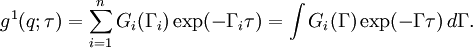
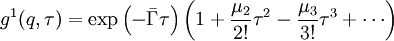
DescriptionWhen light hits small particles the light scatters in all directions (Rayleigh scattering) so long as the particles are small compared to the wavelength (< 250 nm). If the light source is a laser, and thus is monochromatic and coherent, then one observes a time-dependent fluctuation in the scattering intensity. These fluctuations are due to the fact that the small molecules in solutions are undergoing Brownian motion and so the distance between the scatterers in the solution is constantly changing with time. This scattered light then undergoes either constructive or destructive interference by the surrounding particles and within this intensity fluctuation information is contained about the time scale of movement of the scatterers. There are several ways to derive dynamic information about particles’ movement in solution by Brownian motion. One of such methods is dynamic light scattering, also known as quasi elastic laser light scattering. The dynamic information of the particles is derived from an autocorrelation of the intensity trace recorded during the experiment. The second order autocorrelation curve is generated from the intensity trace as follows: where where Data analysisCumulant methodOne of the most common methods is the cumulant method [1] [2], from which in addition to the sum of the exponentials above, more information can be derived about the variance of the system as follows: where with where Depending on the anisotropy and polydispersity of the system, a resulting plot of One must note that the cumulant method is valid for small CONTIN algorithmAn alternative method for analyzing the autocorrelation function can be achieved through an inverse Laplace transform known as CONTIN developed by Steven Provencher.[6].[7] The CONTIN analysis is ideal for heterodisperse, polydisperse and multimodal systems which cannot be resolved with the cumulant method. The resolution for separating two different particle populations is approximately a factor of five or higher and the difference in relative intensities between two different populations should be less than 1 : 1E-5. Maximum entropy methodThe Maximum entropy method is an analysis method that has great developmental potential. The method is also used for the quantification of sedimentation velocity data from analytical ultracentrifugation. The maximum entropy method involves a number of iterative steps to minimize the deviation of the fitted data from the experimental data and subsequently reducing the See also
References
Categories: Fluorescence | Biochemistry methods | Physical chemistry | Spectroscopy | Colloidal chemistry |
|
| This article is licensed under the GNU Free Documentation License. It uses material from the Wikipedia article "Dynamic_light_scattering". A list of authors is available in Wikipedia. |


 is the autocorrelation function at a particular wave vector,
  and delay time,
  and
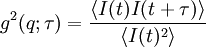
and  is the intensity. At short time delays the correlation is high because the particles do not have a chance to move to a great extent from the initial state that they were in. The two signals are thus essentially unchanged when compared after only a very short time interval. As the time delays become longer, the correlation starts to exponentially fall off to zero, meaning that there is no correlation between the intensity of scattering of the initial state with the final state after a long time period has elapsed (relative to the motion of the particles). This exponential decay is obviously then related to the motion of the particles specifically, the diffusion coefficient. To fit the decay (i.e. the autocorrelation function), numerical methods are used based on calculations of assumed distributions. If the sample was monodisperse the decay would simply be a single exponential. The Siegert equation, relates the second order autocorrelation curve with the first order autocorrelation
  function as follows:
![g^2(q;\tau)= \ 1+\beta\left[g^1(q;\tau)\right]^2](images/math/e/2/9/e29fb022c2fbf44a2663948948708d94.png)
 is a parameter which is a correction factor depending on the geometry and alignment of the laser beam of the light scattering setup; it is roughly equal to the inverse of the number of speckle (see Speckle pattern) from which light is collected. Once the autocorrelation curve has been generated, different mathematical approaches can be employed to fit the curve and thus determine the z-averaged translational diffusion coefficient. The simplest approach is to treat the first order autocorrelation function as the sum of single exponential decays with fractions
  where
where  is the decay rate.
 is the average decay rate and
  is the second order polydispersity index (or an indication of the variance). A third order
  may be derived at a single angle or at a range of angles depending on the wave vector
 is the incident laser wavelength,
  is the refractive index of the sample and
  is angle at which the detector is located with respect to the sample cell.
 vs.
vs.  may or may not show an angular dependence. Spherical particles will show no angular dependence, hence no anisotropy. A plot of
  , because overfitting data with many parameters in a power-series expansion will render all the parameters including
  and
and  , less precise
  of the fitted data.


