To use all functions of this page, please activate cookies in your browser.
My watch list
my.chemeurope.com
my.chemeurope.com
With an accout for my.chemeurope.com you can always see everything at a glance – and you can configure your own website and individual newsletter.
- My watch list
- My saved searches
- My saved topics
- My newsletter
Frequency-resolved optical gatingIn optics, frequency-resolved optical gating (FROG) is a derivative of autocorrelation, but is far superior in its ability to measure ultrafast optical pulse shapes. Further, it can determine the phase of the pulse. In the most common configuration, FROG is simply a background-free autocorrelator followed by a spectrometer. It is the two-dimensional nature of the FROG trace that allows the extraction of the actual pulse shape and phase from the data. Product highlight
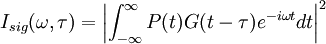
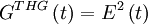
The basicsFrequency-Resolved refers to the fact that the final signal is a spectrum. Before explaining Optical Gating, it helps to recognize that the pulse is really interacting with itself. In most configurations, the pulse is split and recombined, as in an interferometer. However, in this case, the recombination does not occur on a beam-splitter, but rather in a nonlinear medium, which allows the two beams to interact with each other. It is this interaction that allows the pulses to "gate" the spectral information of the other pulse. So Optical Gating refers to the fact that the measured spectrum is really from a time-slice of the pulse, and that time-slice is determined by the pulse nonlinear interaction. The gate function depends on the type of nonlinear interaction allowed. Mathematically the FROG trace is simply a spectrogram but with an unknown gate function: where P(t) is the "probe" pulse and G(t) is the "gate" pulse. The probe and gate pulses are determined by the nonlinear interaction used, and it is the form of the probe and gate that distinguishes the different types of FROG from each other. Some of the most common are:
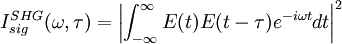
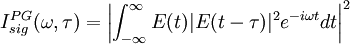
For example second-harmonic generation FROG (SHG FROG) would be: and PG FROG would be: Traditional inversion algorithms for spectrograms requires perfect knowledge of the gate function (G(t)), however, FROG does not have this luxury. Instead an iterative alogrithm is used. The algorithm uses both the data (FROG trace) and form of the nonlinearity to achieve a best match between the real FROG trace and the "retrieved" FROG trace. The retrieved FROG trace is created synthetically from the best guess for E(t). FROG algorithm
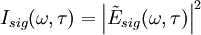
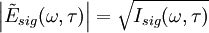
The FROG algorithm is all about phase retrieval. The FROG trace measured in the lab is the exact intensity of Isig(ω,τ); however, it is missing the phase information. To start off with define a signal field: and further defining: given this the FROG trace becomes: inverting this: so the amplitude of An iterative algorithm is used to determine this unknown phase.
See alsoFROG techniques
Competing techniques
Further reading
|
|||||||||||||
| This article is licensed under the GNU Free Documentation License. It uses material from the Wikipedia article "Frequency-resolved_optical_gating". A list of authors is available in Wikipedia. |


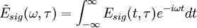
 is known, but not its phase.
If this phase is found, then the pulse (
is known, but not its phase.
If this phase is found, then the pulse ( .
.
 from
from  ). Call this
  .
.
 ).
).
 to
to 

