My watch list

Home
Encyclopedia
Optical_autocorrelation

Optical autocorrelation

In optics, various autocorrelation functions can be experimentally realized. The field autocorrelation may be used to calculate the spectrum of a source of light, while the intensity autocorrelation and the interferometric autocorrelation are commonly used to estimate the duration of ultrashort pulses produced by modelocked lasers. (To accurately and definitively determine the pulse length, one needs to perform a full-intensity-and-phase type of measurement, such as SPIDER or FROG.) The laser pulse duration cannot be easily measured by optoelectronic methods, since the response time of photodiodes and oscilloscopes are at best of the order of 200 femtoseconds.

In the following examples, the autocorrelation signal is generated by second-harmonic generation (SHG), the lowest order (and hence the strongest) of all nonlinear optical processes. Higher-order nonlinear optical processes such as third-harmonic generation can also be used in autocorrelation measurements, in which case the mathematical expressions of the signal will be slightly modified, but the basic interpretation of an autocorrelation trace remains the same.

Additional recommended knowledge

Weighing the right way

Correct Test Weight Handling Guide: 12 Practical Tips

Better weighing performance in 6 easy steps

1 Field autocorrelation
2 Intensity autocorrelation
3 Interferometric autocorrelation
4 Pupil function autocorrelation
5 See also

Field autocorrelation

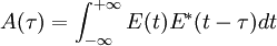
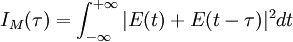
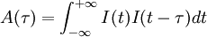
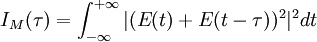
For a complex electric field $E (t)$ , the field autocorrelation function is defined by

$A(\tau) = \int_{-\infty}^{+\infty}E(t)E^*(t-\tau)dt$

The Wiener-Khinchin theorem states that the Fourier transform of the field autocorrelation is the spectrum of $E (t)$ , i.e., the square of the magnitude of the Fourier transform of $E (t)$ . As a result, the field autocorrelation is not sensitive to the spectral phase.

The field autocorrelation is readily measured experimentally by placing a slow detector at the output of a Michelson interferometer. The detector is illuminated by the input electric field $E (t)$ coming from one arm, and by the delayed replica $E (t - τ)$ from the other arm. If the time response of the detector is much larger than the time duration of the signal $E (t)$ , or if the recorded signal is integrated, the detector measures the intensity $I M$ as the delay $τ$ is scanned:

$I_M(\tau) = \int_{-\infty}^{+\infty}|E(t)+E(t-\tau)|^2dt$

Expanding $I M (τ)$ reveals that one of the terms is $A (τ)$ , proving that a Michelson interferometer can be used to measure the field autocorrelation, or the spectrum of $E (t)$ (and only the spectrum). This principle is the basis for Fourier transform spectroscopy.

Intensity autocorrelation

To a complex electric field $E (t)$ corresponds an intensity $I (t) = | E (t) | 2$ and an intensity autocorrelation function defined by

$A(\tau) = \int_{-\infty}^{+\infty}I(t)I(t-\tau)dt$

The optical implementation of the intensity autocorrelation is not as straightforward as for the field autocorrelation. Similarly to the previous setup, two parallel beams with a variable delay are generated, then focused into a second-harmonic-generation crystal (see nonlinear optics) to obtain a signal proportional to $(E (t) + E (t - τ)) 2$ . Only the beam propagating on the optical axis, proportional to the cross-product $E (t) E (t - τ)$ , is retained. This signal is then recorded by a slow detector, which measures

$I_M(\tau) = \int_{-\infty}^{+\infty}|E(t)E(t-\tau)|^2dt = \int_{-\infty}^{+\infty}I(t)I(t-\tau)dt$

$I M (τ)$ is exactly the intensity autocorrelation $A (τ)$ .

The generation of the second harmonic in crystals is a nonlinear process that requires high peak power, unlike the previous setup. However, such high peak power can be obtained from a limited amount of energy by ultrashort pulses, and as a result their intensity autocorrelation is often measured experimentally. Another difficulty with this setup is that both beams must be focused at the same point inside the crystal as the delay is scanned in order for the second harmonic to be generated.

It can be shown that the intensity autocorrelation width of a pulse is related to the intensity width. For a Gaussian time profile, the autocorrelation width is $\sqrt{2}$ longer than the width of the intensity, and it is 1.54 longer in the case of an hyperbolic secant squared (sech²) pulse. This numerical factor, which depends on the shape of the pulse, is sometimes called the deconvolution factor. If this factor is known, or assumed, the time duration (intensity width) of a pulse can be measured using an intensity autocorrelation. However, the phase cannot be measured.

Interferometric autocorrelation

As a combination of both previous cases, a nonlinear crystal can be used to generate the second harmonic at the output of a Michelson interferometer, in a colinear geometry. In this case, the signal recorded by a slow detector is

$I_M(\tau) = \int_{-\infty}^{+\infty}|(E(t)+E(t-\tau))^2|^2dt$

$I M (τ)$ is called the interferometric autocorrelation. It contains some information about the phase of the pulse: the fringes in the autocorrelation trace wash out as the spectral phase becomes more complex.

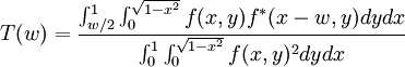
Pupil function autocorrelation

The optical transfer function T(w) of an optical system is given by the autocorrelation of its pupil function f(x,y):

$T(w) = \frac{\int_{w/2}^{1} \int_{0}^{\sqrt{1-x^2}} f(x,y) f^*(x-w,y)dy dx}{\int_{0}^{1}\int_{0}^{\sqrt{1-x^2}}f(x,y)^2 dy dx}$

Optical autocorrelation

Additional recommended knowledge

Weighing the right way

Correct Test Weight Handling Guide: 12 Practical Tips

Better weighing performance in 6 easy steps

Contents

Field autocorrelation

Intensity autocorrelation

Interferometric autocorrelation

Pupil function autocorrelation

See also

About chemeurope.com

About LUMITOS

Advertise with LUMITOS