To use all functions of this page, please activate cookies in your browser.
My watch list
my.chemeurope.com
my.chemeurope.com
With an accout for my.chemeurope.com you can always see everything at a glance – and you can configure your own website and individual newsletter.
- My watch list
- My saved searches
- My saved topics
- My newsletter
Godunov's theoremProfessor Sergei K. Godunov's most influential work is in the area of applied and numerical mathematics. It has had a major impact on science and engineering, particularly in the development of methodologies used in Computational Fluid Dynamics (CFD) and other computational fields. One of his major contributions was to prove the theorem (Godunov, 1954; Godunov, 1959), that bears his name. Godunov's theorem, also known as Godunov's order barrier theorem states that:
The theorem was originally proved by Godunov as a Ph.D. student at Moscow State University and has been extremely important in the development of the theory of high resolution schemes for the numerical solution of PDEs. Product highlight
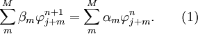
The theoremWe generally follow Wesseling (2001). Aside Assume a continuum problem described by a PDE is to be computed using a numerical scheme based upon a uniform computational grid and a one-step, constant step-size, M grid point, integration algorithm, either implicit or explicit. Then if It is assumed that
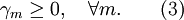
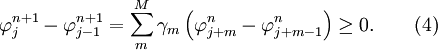
The above scheme of equation (2) is monotonicity preserving if and only if
Assume (3) applies and that Then, because This means that monotonicity is preserved for this case.
For the same monotonically increasing
Linear one-step second-order accurate numerical schemes for the convection equation cannot be monotonicity preserving unless where
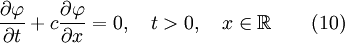
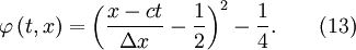
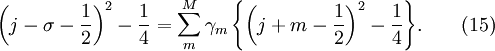
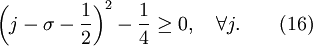
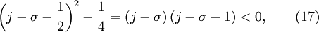
The exact solution is If we assume the scheme to be at least second-order accurate, it should produce the following solution exactly Substituting into equation (2) gives: Suppose that the scheme IS monotonicity preserving, then according to the theorem 1 above, Now, it is clear from equation (15) that Assume It therefore follows that, which contradicts equation (16) and completes the proof. The exceptional situation whereby References
Further reading
See also |
|
| This article is licensed under the GNU Free Documentation License. It uses material from the Wikipedia article "Godunov's_theorem". A list of authors is available in Wikipedia. |


 and
and  , such a scheme can be described by
 determines
  uniquely. Now, since the above equation represents a linear relationship between
  and
and 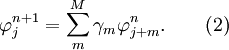
 is monotonically increasing with
  .
.
 it therefore follows that
 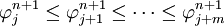 because
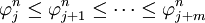
 , assume that
  for some
  and choose

![\varphi _j^{n + 1} - \varphi _{j-1}^{n+1} = \sum\limits_m^M {\gamma _m } \left( {\varphi _{j + m}^{n} - \varphi _{j + m - 1}^{n} } \right) = \left\{ {\begin{array}{*{20}c} {0,} & {\left[ {j + m \ne k} \right]} \\ {\gamma _m ,} & {\left[ {j + m = k} \right]} \\ \end{array}} \right . \quad \quad ( 6)](images/math/c/e/0/ce0ac9e056c71c1d352f261c85678589.png)
 , to give

 , which completes the proof.
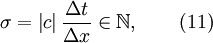
 is the signed Courant–Friedrichs–Lewy condition (CFL) number.


 .
.
 and choose
  . This implies that
  and
and  .
.
 is only of theoretical interest, since this cannot be realised with variable coefficients. Also, integer CFL numbers greater than unity would not be feasible for practical problems.


