Flux limiters are used in high resolution schemes — numerical schemes used to solve problems in science and engineering, particularly fluid dynamics, described by partial differential equations (PDE's). They are used in high resolution schemes, such as the MUSCL scheme, to avoid the spurious oscillations (wiggles) that would otherwise occur with high order spatial discretisation schemes due to shocks, discontinuities or sharp changes in the solution domain. Use of flux limiters, together with an appropriate high resolution scheme, make the solutions total variation diminishing (TVD).
Note:
Flux limiters are also referred to as slope limiters because they both have the same mathematical form, and both have the effect of limiting the solution gradient near shocks or discontinuities. In general, the term flux limiter is used when the limiter acts on system fluxes, and slope limiter is used when the limiter acts on system states.
How they work
The main idea behind the construction of flux limiter schemes is to limit the spatial derivatives to realistic values - for scientific and engineering problems this usually means physically realisable values. They are used in high resolution schemes for solving problems described by PDE's and only come into operation when sharp wave fronts are present. For smoothly changing waves, the flux limiters do not operate and the spatial derivatives can be represented by higher order approximations without introducing non-real oscillations. Consider the 1D semi-discrete scheme below,
![\frac{d u_i}{d t} + \frac{1}{\Delta x_i} \left[ F \left( u_{i + \frac{1}{2}} \right) - F \left( u_{i - \frac{1}{2}} \right) \right] =0](images/math/9/3/0/93033b6e2189976d69743b2de8a13c8c.png) . .
where,  and and  represent edge fluxes for the ith cell. If these edge fluxes can be represented by low and high resolution schemes, then a flux limiter can switch between these schemes depending upon the gradients close to the particular cell, as follows, represent edge fluxes for the ith cell. If these edge fluxes can be represented by low and high resolution schemes, then a flux limiter can switch between these schemes depending upon the gradients close to the particular cell, as follows,
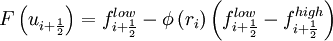 , ,
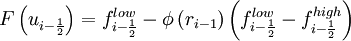 , ,
where,
 low resolution flux, low resolution flux,
 high resolution flux, high resolution flux,
 flux limiter function, flux limiter function,
and  represents the ratio of successive gradients on the solution mesh, i.e., represents the ratio of successive gradients on the solution mesh, i.e.,
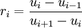 . .
The limiter function is constrained to be greater than or equal to zero, i.e.,  . Therefore, when the limiter is equal to zero (sharp gradient, opposite slopes or zero gradient), the flux is represented by a low resolution scheme. Similarly, when the limiter is equal to 1 (smooth solution), it is represented by a high resolution scheme. The various limiters have differing switching characteristics and are selected according to the particular problem and solution scheme. No particular limiter has been found to work well for all problems, and a particular choice is usually made on a trial and error basis. . Therefore, when the limiter is equal to zero (sharp gradient, opposite slopes or zero gradient), the flux is represented by a low resolution scheme. Similarly, when the limiter is equal to 1 (smooth solution), it is represented by a high resolution scheme. The various limiters have differing switching characteristics and are selected according to the particular problem and solution scheme. No particular limiter has been found to work well for all problems, and a particular choice is usually made on a trial and error basis.
Limiter functions
The following are common forms of flux/slope limiter function,  : :
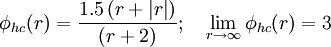
CHARM [not 2nd order TVD] (Zhou, 1995)
 . .
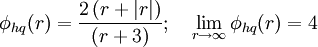
HCUS [not 2nd order TVD] (Waterson & Deconinck, 1995)
 . .
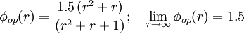
HQUICK [not 2nd order TVD] (Waterson & Deconinck, 1995)
 . .
Koren (Koren, 1993)
![\phi_{kn}(r) = \max \left[ 0, \min \left(2 r, \left(1+2r \right)/3, 2 \right) \right]; \quad \lim_{r \rightarrow \infty}\phi_{kn}(r) = 2](images/math/f/5/5/f55d585d5df8dd0b2beebebdeb061357.png) . .
minmod - symmetric (Roe, 1986)
![\phi_{mm} (r) = \max \left[ 0 , \min \left( 1 , r \right) \right] ; \quad \lim_{r \rightarrow \infty}\phi_{mm}(r) = 1](images/math/4/e/4/4e41a9e0f757cf73101f7d4d7bc7fcdd.png) . .
monotonized central (MC) - symmetric (van Leer, 1977)
![\phi_{mc} (r) = \max \left[ 0 , \min \left( 2 r, 0.5 (1+r), 2 \right) \right] ; \quad \lim_{r \rightarrow \infty}\phi_{mc}(r) = 2](images/math/a/7/d/a7dade97ef273a70ebb4142807db9c00.png) . .
Osher (Chatkravathy and Osher, 1983)
![\phi_{os} (r) = \max \left[ 0 , \min \left( r, \beta \right) \right], \quad \left(1 \leq \beta \leq 2 \right) ; \quad \lim_{r \rightarrow \infty}\phi_{os} (r) = \beta](images/math/c/f/6/cf63b9d57a3bc1d059dac0da831b6eab.png) . .
ospre - symmetric (Waterson & Deconinck, 1995)
 . .
smart [not 2nd order TVD] (Gaskell & Lau, 1988)
![\phi_{sm}(r) = \max \left[ 0, \min \left(2 r, \left(0.25 + 0.75 r \right), 4 \right) \right] ; \quad \lim_{r \rightarrow \infty}\phi_{sm}(r) = 4](images/math/5/d/1/5d1711c027f4da08a7adecfc59d701c6.png) . .
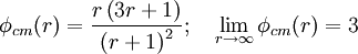
superbee - symmetric (Roe, 1986)
![\phi_{sb} (r) = \max \left[ 0, \min \left( 2 r , 1 \right), \min \left( r, 2 \right) \right] ; \quad \lim_{r \rightarrow \infty}\phi_{sb} (r) = 2](images/math/e/5/1/e510b5a7afa1c72648712d4756d52a10.png) . .
Sweby - symmetric (Sweby, 1984)
![\phi_{sw} (r) = \max \left[ 0 , \min \left( \beta r, 1 \right), \min \left( r, \beta \right) \right], \quad \left(1 \leq \beta \leq 2 \right) ; \quad \lim_{r \rightarrow \infty}\phi_{sw} (r) = \beta](images/math/7/b/4/7b44b55c6730737b6c0e835bf5ecc3ef.png) . .
UMIST (Lien & Leschziner, 1994)
![\phi_{um}(r) = \max \left[ 0, \min \left(2 r, \left(0.25 + 0.75 r \right), \left(0.75 + 0.25 r \right), 2 \right) \right] ; \quad \lim_{r \rightarrow \infty}\phi_{um}(r) = 2](images/math/b/7/3/b7336e77ef6cabe746c015bfe86af87c.png) . .
van Albada 1 - symmetric (van Albada, et al, 1982)
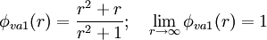 . .
van Albada 2 Alternative form [not 2nd order TVD] used on high spatial order schemes (Kermani, 2003)
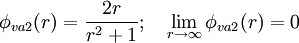 . .
van Leer - symmetric (van Leer, 1974)
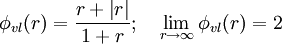 . .
All the above limiters indicated as being symmetric, exhibit the following symmetry property,
 . .
This is a desirable property as it ensures that the limiting actions for forward and backward gradients operate in the same way.
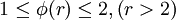
Unless indicated to the contrary, the above limiter functions are second order TVD. This means that they are designed such that they pass through a certain region of the solution, known as the TVD region, in order to guarantee stability of the scheme. Second-order, TVD limiters satisfy at least the following criteria:
The admissible limiter region for second-order TVD schemes is shown in the Sweby Diagram opposite (Sweby, 1984), and plots showing limiter functions overlaid onto the TVD region are shown below. In this image, plots for the Osher and Sweby limiters have been generated using β = 1.5.
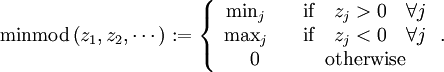
Generalised mimmod limiter
An additional limiter that has an interesting form is the generalised minmod limiter (Harten and Osher, 1987). It is defined as follows
![\phi_{mg}(u,\theta)=\textrm{minmod}\left(\theta\frac{u_{i}-u_{i-1}}{\Delta x},\;\frac{u_{i+1}-u_{i-1}}{2\Delta x},\;\theta\frac{u_{i+1}-u_{i}}{\Delta x}\right),\quad\theta\in\left[1,2\right],](images/math/7/2/d/72d6c9759a583de2f2ae654ff4cc5a23.png)
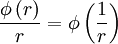
where
Note:  is most dissipative for is most dissipative for  when it reduces to when it reduces to  and is least dissipative for and is least dissipative for  . .
See also
References
- Chatkravathy, S R and S Osher, (1983), High resolution applications of the Osher upwind scheme for the Euler equations, AIAA Paper 83-1943, Proc. AIAA 6th Comutational Fluid Dynamics Conference, pp 363-73.
- Gaskell, P H and A K C Lau, (1988), Curvature-compensated convective transport: SMART, a new boundedness-preserving transport algorithm, Int. J. Num. Meth. Fluids, 8, p617.
- Harten, A. and S. Osher, (1987). Uniformly high-order accurate nonoscillatory schemes. I, SIAM J. Numer. Anal., 24, pp. 279–309.
- Hirsch, C, (1990), Numerical Computation of Internal and External Flows, volume 2: Computational Methods for Inviscid and Viscous Flows, Wiley.
- Kermani, M. J., Gerber, A. G., and Stockie, J. M. (2003), Thermodynamically Based Moisture Prediction Using Roe’s Scheme, 4th Conference of Iranian AeroSpace Society, Amir Kabir University of Technology, Tehran, Iran, January 27–29.
- Koren, B, (1993), A robust upwind discretisation method for advection, diffusion and source terms, In: Numerical Methods for Advection-Diffusion Problems, Ed. C.B.Vreugdenhil & B.Koren, Vieweg, Braunschweig, p117.
- Leonard, B P, M A Leschziner and J McGuirk, (1978), The QUICK algorithm: a uniformly 3rd-order finite-difference method for highly convective flows, Proc. 1st Conf. on Numerical Methods in Laminar & Turbulent Flow, Swansea, p807.
- Lien, F S, and M. A. Leschziner, (1994), Upstream monotonic interpolation for scalar transport with application to complex turbulent flows, Int. J. Num. Meth. Fluids, 19, p527.
- Roe, P L, (1986), Characteristic-based schemes for the Euler equations, Ann. Rev. Fluid Mech., 18, p337.
- Sweby, P K, (1984), High resolution schemes using flux-limiters for hyperbolic conservation laws. SIAM J. Num. Anal., 21, p995-1011.
- Van Albada, G D, B. Van Leer and W. W. Roberts, (1982), A comparative study of computational methods in cosmic gas dynamics, Astron. Astrophysics, 108, p76.
- Van Leer, B, (1974), Towards the ultimate conservative difference scheme II. Monotonicity and conservation combined in a second order scheme. J. Comp. Phys., 14, p361-70.
- Van Leer, B, (1977), Towards the ultimate conservative difference scheme III. Upstream-centered finite-difference schemes for ideal compressible flow., J. Comp. Phys., 23, p263-75.
- Van Leer, B, (1979), Towards the ultimate conservative difference scheme V, J. Comp. Phys., 32, p101.
- Waterson, N P and H Deconinck, (1995), A unified approach to the design and application of bounded higher-order convection schemes, VKI Preprint 1995-21.
- Zhou, G, (1995), Numerical simulations of physical discontinuities in single and multi-fluid flows for arbitrary Mach numbers, PhD Thesis, Chalmers Univ. of Tech., Goteborg, Sweden.
Further reading
- Hirsch, C. (1990), Numerical Computation of Internal and External Flows, Volume 2: Computational Methods for Inviscid and Viscous Flows, Wiley.
- Laney, Culbert B. (1998), Computational Gas Dynamics, Cambridge University Press.
- LeVeque, Randall (1990), Numerical Methods for Conservation Laws, ETH Lectures in Mathematics Series, Birkhauser-Verlag.
- LeVeque, Randall (2002), Finite Volume Methods for Hyperbolic Problems, Cambridge University Press.
- Toro, E. F. (1999), Riemann Solvers and Numerical Methods for Fluid Dynamics, Springer-Verlag.
- Tannehill, John C., et al, (1997), Computational Fluid mechanics and Heat Transfer, 2nd Ed., Taylor and Francis.
- Wesseling, Pieter (2001), Principles of Computational Fluid Dynamics, Springer-Verlag.
|


 ,
,
 ,
,
 ,
,
 ,
,


