My watch list

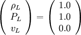
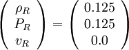
Sod Shock Tube

The Sod Shock Tube problem, named after Gary A. Sod, is a common test for the accuracy of computational fluid codes, like Riemann solvers, and was heavily investigated by Sod in 1978.

Additional recommended knowledge

How to ensure accurate weighing results every day?

How to quickly check pipettes?

Daily Sensitivity Test

The test consist of an one dimensional Riemann problem with the following paramters, for left and right states of an ideal gas.

$\left( \begin{array}{c}\rho_L\\P_L\\v_L\end{array}\right) = \left( \begin{array}{c}1.0\\1.0\\0.0\end{array} \right)$ , $\left( \begin{array}{c}\rho_R\\P_R\\v_R\end{array}\right) = \left( \begin{array}{c}0.125\\0.125\\0.0\end{array}\right)$

where

$ρ$ is the density
P is the pressure
v is the velocity

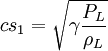
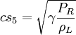
The time evolution of this problem can be described by solving the Euler equations. Which leads to three characteristics, describing the propagation speed of the various regions of the system. Namely the rarefaction wave, the contact discontinuity and the shock discontinuity. If this is solved numerically, one can test against the analytical solution, and get information how good a code captures and resolves shocks and contact discontinuities and reproduce the correct density profile of the rarefaction wave.

Analytic derivation

The different state of the solution are separated by the time evolution of the three characteristics of the system, which is due to the finite speed of information propagation. Two of them are equal to the speed of sound of the both states

$cs_1 = \sqrt{\gamma \frac{P_L}{\rho_L}}$

$cs_5 = \sqrt{\gamma \frac{P_R}{\rho_L}}$

The first one is the position of the beginning of the rarefaction wave while the other the velocity of the propagation of the shock.

Defining:

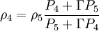
$\Gamma = \frac{\gamma - 1}{\gamma + 1}$ , $\beta = \frac{\gamma - 1}{2 \gamma}$

The states after the shock are connected by the Rankine Hugoniot shock jump conditions.

$\rho_4 = \rho_5 \frac{P_4 + \Gamma P_5}{P_5 + \Gamma P_4}$

But to calculate the denisty in Region 4 we need to know the pressure in that region. This is related by the contact discontinuity with the pressure in region 3 by

P 4 = P 3

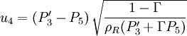
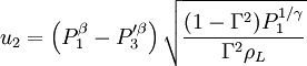
Unfortunately the pressure in region 3 can only be calculated interatively, the right solution is found when $u 2$ equals $u 4$

$u_4 = \left(P_3' - P_5\right)\sqrt{\frac{1-\Gamma}{\rho_R(P_3'+\Gamma P_5)}}$

$u_2 =\left(P_1^\beta-P_3'^\beta\right) \sqrt{\frac{(1-\Gamma^2)P_1^{1/\gamma}}{\Gamma^2 \rho_L}}$

u 2 - u 4

This function can be evaluated to an arbitrary precision thus giving the pressure in the region 3

P 3 = c a l c u l a t e (P 3, s, s,,)

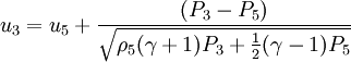
finally we can calulcate

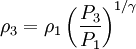
$u_3 = u_5 + \frac{(P_3 - P_5)}{\sqrt{\rho_5(\gamma+1)P_3 +\frac{1}{2}(\gamma-1)P_5}}$

u 4 = u 3

and $ρ 3$ follows from the adiabatic gas law

$\rho_3 = \rho_1 \left(\frac{P_3}{P_1}\right)^{1/\gamma}$

References

Sod, G. A. (1978). "A Survey of Several Finite Difference Methods for Systems of Nonlinear Hyperbolic Conservation Laws". J. Comput. Phys. 27: 1–31.
Toro, Eleuterio F. (1999). Riemann Solvers and Numerical Methods for Fluid Dynamics. Berlin: Springer Verlag. ISBN 3-540-65966-8.

Sod Shock Tube

Additional recommended knowledge

How to ensure accurate weighing results every day?

How to quickly check pipettes?

Daily Sensitivity Test

Analytic derivation

References

See also

About chemeurope.com

About LUMITOS

Advertise with LUMITOS