To use all functions of this page, please activate cookies in your browser.
My watch list
my.chemeurope.com
my.chemeurope.com
With an accout for my.chemeurope.com you can always see everything at a glance – and you can configure your own website and individual newsletter.
- My watch list
- My saved searches
- My saved topics
- My newsletter
Computational fluid dynamicsComputational fluid dynamics (CFD) is one of the branches of fluid mechanics that uses numerical methods and algorithms to solve and analyze problems that involve fluid flows. Computers are used to perform the millions of calculations required to simulate the interaction of fluids and gases with the complex surfaces used in engineering. However, even with simplified equations and high-speed supercomputers, only approximate solutions can be achieved in many cases. More accurate software that can accurately and quickly simulate even complex scenarios such as transonic or turbulent flows are an ongoing area of research. Validation of such software is often performed using a wind tunnel. Product highlight
Background and historyThe fundamental basis of any CFD problem are the Navier-Stokes equations, which define any single-phase fluid flow. These equations can be simplified by removing terms describing viscosity to yield the Euler equations. Further simplification, by removing terms describing vorticity yields the full potential equations. Finally, these equations can be linearized to yield the linearized potential equations. Historically, methods were first developed to solve the Linearized Potential equations. Two-dimensional methods, using conformal transformations of the flow about a cylinder to the flow about an airfoil were developed in the 1930s. The computer power available paced development of three-dimensional methods. The first paper on a practical three-dimensional method to solve the linearized potential equations was published by John Hess and A.M.O. Smith of Douglas Aircraft in 1966. This method discretized the surface of the geometry with panels, giving rise to this class of programs being called Panel Methods. Their method itself was simplified, in that it did not include lifting flows and hence was mainly applied to ship hulls and aircraft fuselages. The first lifting Panel Code (A230) was described in a paper written by Paul Rubbert and Gary Saaris of Boeing Aircraft in 1968. In time, more advanced three-dimensional Panel Codes were developed at Boeing (PANAIR, A502), Lockheed (Quadpan), Douglas (HESS), McDonnell Aircraft (MACAERO), NASA(PMARC) and Analytical Methods (WBAERO, USAERO and VSAERO). Some (PANAIR, HESS and MACAERO) were higher order codes, using higher order distributions of surface singularities, while others (Quadpan, PMARC, USAERO and VSAERO) used single singularities on each surface panel. The advantage of the lower order codes was that they ran much faster on the computers of the time. Today, VSAERO has grown to be a multi-order code and is the most widely used program of this class. This program has been used in the development of many submarines, surface ships, automobiles, helicopters and aircraft. Its sister code, USAERO is an unsteady panel method that has also been used for modeling such things as high speed trains and racing yachts. The NASA PMARC code was developed from an early version of VSAERO and a derivative of PMARC, named CMARC, is also commercially available. In the two-dimensional realm, quite a number of Panel Codes have been developed for airfoil analysis and design. These codes typically have a boundary layer analysis included, so that viscous effects can be modeled. Professor Richard Eppler of the University of Stuttgart developed the PROFIL code, partly with NASA funding, which became available in the early 1980s. This was soon followed by MIT Professor Mark Drela's Xfoil code. Both PROFIL and Xfoil incorporate two-dimensional panel codes, with coupled boundary layer codes for airfoil analysis work. PROFIL uses a conformal transformation method for inverse airfoil design, while Xfoil has both a conformal transformation and an inverse panel method for airfoil design. Both codes are widely used. An intermediate step between Panel Codes and Full Potential codes were codes that used the Transonic Small Disturbance equations. In particular, the three-dimensional WIBCO code, developed by Charlie Boppe of Grumman Aircraft in the early 1980s has seen heavy use. Developers next turned to Full Potential codes, as panel methods could not calculate the non-linear flow present at transonic speeds. The first description of a means of using the Full Potential equations was published by Earll Murman and Julian Cole of Boeing in 1970. Frances Bauer, Paul Garabedian and David Korn of the Courant Institute at New York University (NYU) wrote a series of two-dimensional Full Potential airfoil codes that were widely used, the most important being named Program H. A further growth of Progam H was developed by Bob Melnik and his group at Grumman Aerospace as Grumfoil. Antony Jameson, originally at Grumman Aircraft and the Courant Institute of NYU, worked with David Caughey to develop the important three-dimensional Full Potential code FLO22 in 1975. Many Full Potential codes emerged after this, culminating in Boeing's Tranair (A633) code, which still sees heavy use. The next step was the Euler equations, which promised to provide more accurate solutions of transonic flows. The methodology used by Jameson in his three-dimensional FLO57 code (1981) was used by others to produce such programs as Lockheed's TEAM program and IAI/Analytical Methods' MGAERO program. MGAERO is unique in being a structured cartesian mesh code, while most other such codes use structured body-fitted grids (with the exception of NASA's highly successful CART3D code, Lockheed's SPLITFLOW code and Georgia Tech's NASCART-GT).[1] Antony Jameson also developed the three-dimensional AIRPLANE code (1985) which made use of unstructured tetrahedral grids. In the two-dimensional realm, Mark Drela and Michael Giles, then graduate students at MIT, developed the ISES Euler program (actually a suite of programs) for airfoil design and analysis. This code first became available in 1986 and has been further developed to design, analyze and optimize single or multi-element airfoils, as the MSES program. MSES sees wide use throughout the world. A derivative of MSES, for the design and analysis of airfoils in a cascade, is MISES, developed by Harold "Guppy" Youngren while he was a graduate student at MIT. The Navier-Stokes equations were the ultimate target of developers. Two-dimensional codes, such as NASA Ames' ARC2D code first emerged. A number of three-dimensional codes were developed (OVERFLOW, CFL3D are two successful NASA contributions), leading to numerous commercial packages. TechnicalitiesThe most fundamental consideration in CFD is how one treats a continuous fluid in a discretized fashion on a computer. One method is to discretize the spatial domain into small cells to form a volume mesh or grid, and then apply a suitable algorithm to solve the equations of motion (Euler equations for inviscid, and Navier-Stokes equations for viscous flow). In addition, such a mesh can be either irregular (for instance consisting of triangles in 2D, or pyramidal solids in 3D) or regular; the distinguishing characteristic of the former is that each cell must be stored separately in memory. Where shocks or discontinuities are present, high resolution schemes such as Total Variation Diminishing (TVD), Flux Corrected Transport (FCT), Essentially NonOscillatory (ENO), or MUSCL schemes are needed to avoid spurious oscillations (Gibbs phenomenon) in the solution. If one chooses not to proceed with a mesh-based method, a number of alternatives exist, notably :
It is possible to directly solve the Navier-Stokes equations for laminar flows and for turbulent flows when all of the relevant length scales can be resolved by the grid (a Direct numerical simulation). In general however, the range of length scales appropriate to the problem is larger than even today's massively parallel computers can model. In these cases, turbulent flow simulations require the introduction of a turbulence model. Large eddy simulations (LES) and the Reynolds-averaged Navier-Stokes equations (RANS) formulation, with the k-ε model or the Reynolds stress model, are two techniques for dealing with these scales. In many instances, other equations (mostly convective-diffusion equations) are solved simultaneously with the Navier-Stokes equations. These other equations can include those describing species concentration, chemical reactions, heat transfer, etc. More advanced codes allow the simulation of more complex cases involving multi-phase flows (eg, liquid/gas, solid/gas, liquid/solid) or non-Newtonian fluids (such as blood). MethodologyIn all of these approaches the same basic procedure is followed.
Discretization methodsThe stability of the chosen discretization is generally established numerically rather than analytically as with simple linear problems. Special care must also be taken to ensure that the discretization handles discontinuous solutions gracefully. The Euler equations and Navier-Stokes equations both admit shocks, and contact surfaces. Some of the discretization methods being used are:
Turbulence modelsTurbulent flow produces fluid interaction at a large range of length scales. This problem means that it is required that for a turbulent flow regime calculations must attempt to take this into account by modifying the Navier-Stokes equatons. Failure to do so may result in an unsteady simulation. When solving the turbulence model there exists a trade-off between accuracy and speed of computation. Direct numerical simulationDirect numerical simulation (DNS) captures all of the relevant scales of turbulent motion, so no model is needed for the smallest scales. This approach is extremely expensive, if not intractable, for complex problems on modern computing machines, hence the need for models to represent the smallest scales of fluid motion. Reynolds-averaged Navier-StokesReynolds-averaged Navier-Stokes equations (RANS) is the oldest approach to turbulence modeling. An ensemble version of the governing equations is solved, which introduces new apparent stresses known as Reynolds stresses. This adds a second order tensor of unknowns for which various models can provide different levels of closure. It is a common misconception that the RANS equations do not apply to flows with a time-varying mean flow because these equations are 'time-averaged'. In fact, statistically unsteady (or non-stationary) flows can equally be treated. This is sometimes referred to as URANS. There is nothing inherent in Reynolds averaging to preclude this, but the turbulence models used to close the equations are valid only as long as the time over which these changes in the mean occur is large compared to the time scales of the turbulent motion containing most of the energy. RANS models can be divided into two broad approaches:
Large eddy simulationLarge eddy simulations (LES) is a technique in which the smaller eddies are filtered and are modeled using a sub-grid scale model, while the larger energy carrying eddies are simulated. This method generally requires a more refined mesh than a RANS model, but a far coarser mesh than a DNS solution. Detached eddy simulationDetached eddy simulations (DES) is a modification of a RANS model in which the model switches to a subgrid scale formulation in regions fine enough for LES calculations. Regions near solid boundaries and where the turbulent length scale is less than the maximum grid dimension are assigned the RANS mode of solution. As the turbulent length scale exceeds the grid dimension, the regions are solved using the LES mode. Therefore the grid resolution is not as demanding as pure LES, thereby considerably cutting down the cost of the computation. Though DES was initially formulated for the Spalart-Allmaras model (Spalart et al, 1997), it can be implemented with other RANS models (Strelets, 2001), by appropriately modifying the length scale which is explicitly or implicitly involved in the RANS model. So while Spalart-Allmaras model based DES acts as LES with a wall model, DES based on other models (like two equation models) behave as a hybrid RANS-LES model. Grid generation is more complicated than for a simple RANS or LES case due to the RANS-LES switch. DES is a non-zonal approach and provides a single smooth velocity field across the RANS and the LES regions of the solutions. Vortex methodThe Vortex method is a grid-free technique for the simulation of turbulent flows. It uses vortices as the computational elements, mimicking the physical structures in turbulence. Vortex methods were developed as a grid-free methodology that would not be limited by the fundamental smoothing effects associated with grid-based methods. To be practical, however, vortex methods require means for rapidly computing velocities from the vortex elements – in other words they require the solution to a particular form of the N-body problem (in which the motion of N objects is tied to their mutual influences). A long-sought breakthrough came in the late 1980’s with the development of the Fast Multipole Method (FMM), an algorithm that has been heralded as one of the top ten advances in numerical science of the 20th century. This breakthrough paved the way to practical computation of the velocities from the vortex elements and is the basis of successful algorithms. Software based on the Vortex method offer the engineer a new means for solving tough fluid dynamics problems with minimal user intervention. All that is required is specification of problem geometry and setting of boundary and initial conditions. Among the significant advantages of this modern technology;
Solution algorithmsThe basic solution of the system of equations arising after discretization is accomplished by many of the familiar algorithms of numerical linear algebra. One can either use a stationary iterative method, like symmetric Gauss-Seidel or successive overrelaxation, or a Krylov subspace method. In the latter, the solution residual is minimized on an orthogonal basis for a subspace of the non-linear operator. Krylov subspace methods are generally used with a preconditioner and an inner Newton iteration. Unfortunately for non-linear problems, the orthogonal basis cannot be constructed with short recurrences (as in the plain conjugate gradient method) and the entire sequence of vectors must be stored. See also
References
Categories: Computational fluid dynamics | Fluid dynamics |
|
| This article is licensed under the GNU Free Documentation License. It uses material from the Wikipedia article "Computational_fluid_dynamics". A list of authors is available in Wikipedia. |


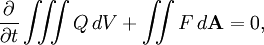
 is the cell surface area.