To use all functions of this page, please activate cookies in your browser.
My watch list
my.chemeurope.com
my.chemeurope.com
With an accout for my.chemeurope.com you can always see everything at a glance – and you can configure your own website and individual newsletter.
- My watch list
- My saved searches
- My saved topics
- My newsletter
Steady state (chemistry)
In chemistry, a steady state is a situation in which all state variables are constant in spite of ongoing processes that strive to change them. For an entire system to be at steady state, i.e. for all state variables of a system to be constant, there must be a flow through the system (compare mass balance). One of the most simple examples of such a system is the the case of a bathtub with the tap open but without the bottom plug: after a certain time the water flows in and out at the same rate, so the water level (the state variable being Volume) stabilises and the system is at steady state. The steady state concept is different from chemical equilibrium. Although both may create a situation where a concentration does not change, in a system at chemical equilibrium, the net reaction rate is zero (products transform into reactants at the same rate as reactants transform into products), while no such limitation exist in the steady state concept. Indeed, there does not have to be a reaction at all for a steady state to develop. The term steady state is also used to describe a situation where some, but not all, of the state variables of a system are constant. For such a steady state to develop, the system does not have to be a flow system. Therefore such a steady state can develop in a closed system where a series of chemical reactions take place. Literature in chemical kinetics usually refers to this case, calling it steady state approximation. In simple systems the steady state is approached by state variables gradually decreasing or increasing until they reach their steady state value. In more complex systems state variable might fluctuate around the theoretical steady state either forever (a limit-cycle) or gradually coming closer and closer. It theoretically takes an infinite time to reach steady state, just as it takes an infinite time to reach chemical equilibrium. Both concepts are, however, frequently used approximations because of the substantial mathematical simplifications these concepts offer. Whether or not these concepts can be used depends on the error the underlying assumptions introduce. So, even though a steady state, from a theoretical point of view, requires constant drivers (e.g. constant inflow rate and constant concentrations in the inflow), the error introduced by assuming steady state for a system with non-constant drivers may be negligible if the steady state is approached fast enough (relatively speaking). Product highlight
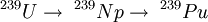
Steady state approximation in chemical kineticsThe steady state approximation[1] involves setting the rate of change of a reaction intermediate in a reaction mechanism equal to zero. It is important to note that steady state approximation does not assume the reaction intermediate concentration to be constant (and therefore its time derivative being zero), it assumes that the variation in the concentration of the intermediate is almost zero: the concentration of the intermediate is very low, so even a big relative variation in its concentration is small, if considered quantitatively. Its use facilitates the resolution of the differential equations that arise from rate equations, which lack an analytical solution for most mechanisms beyond the most simple ones. The steady state approximation is applied, for example in Michaelis-Menten kinetics. As an example, the steady state approximation will be applied to two consecutive, irreversible, homogeneous first order reactions in a closed system. (For heterogeneous reactions, see reactions on surfaces.) This model corresponds, for example, to a series of nuclear decompositions like If the rate constants for the following reaction are k1 and k2; Reaction ratesFor reactant A: For reactant B: For reactant C: Analytical SolutionsThe analytical solutions for these equations (supposing that initial concentrations of every substance except for A are zero) are:
Steady StateIf the steady state approximation is applied then, the derivative of the concentration of the intermediate is set to zero.
ValidityThe analytical and approximated solutions should now be compared in order to decide when it is valid to use the steady state approximation. The analytical solution transforms into the approximate one when The graphs show concentrations of A (red), B (green) and C (blue) in two cases, calculated from the analytical solution:
The equilibrium approximation can be used sometimes in chemical kinetics to yield similar results as the steady state approximation (Michaelis-Menten kinetics can be derived assuming equilibrium instead of steady state): it consists in assuming that the intermediate is at chemical equilibrium. Normally the requirements for applying the steady state approximation are laxer: the concentration of the intermediate is only needed to be low and more or less constant (as seen, this has to do only with the rates at which it appears and disappears) but it is not needed to be at equilibrium, which is usually difficult to prove and involves heavier assumptions.
Notes and references
P. W. Atkins "Physical Chemistry" For a complete derivation of the exact and approximate solution and a comparison between them See alsoCategories: Chemical kinetics | Physical chemistry |
|
| This article is licensed under the GNU Free Documentation License. It uses material from the Wikipedia article "Steady_state_(chemistry)". A list of authors is available in Wikipedia. |


 .
.
 , combining the
 ![\frac{d[A]}{dt} = -k_1 [A]](images/math/8/6/e/86e24b62bbf0b6d0c81b6ff5143b8ab9.png)
![\frac{d[B]}{dt} = k_1 [A] - k_2 [B]](images/math/d/d/b/ddbf39f88d2aea78c65e997ae87434ae.png)
![\frac{d[C]}{dt} = k_2 [B]](images/math/3/9/b/39b9e2213ec97994c460c034d38c59ae.png)
![[A]=[A]_0 e^{-k_1 t}](images/math/7/2/5/7256d2c1532cc5805adcedb96279b69a.png)
![[B]=[A]_0 \frac{k_1}{k_2 - k_1}\left ( e^{-k_1t}-e^{-k_2t} \right )](images/math/c/0/0/c00ef757f86b0d88f333f3b279dfca07.png)
![[C] = \frac{[A]_0}{k_2-k_1} \left [ k_2 \left ( 1- e^{-k_1t} \right ) - k_1 \left (1- e^{-k_2t} \right ) \right ] \quad = [A]_0 \left (1 + \frac{k_1 e^{-k_2t}-k_2e^{-k_1t}}{k_2-k_1} \right )](images/math/1/8/a/18a1c0f713c9f7485d1d81deb0de0517.png)
![\frac{d[B]}{dt} = 0 = k_1 [A] - k_2 [B] \Rightarrow \; [B] = \frac{k_1}{k_2} [A]](images/math/a/f/5/af5ef4d69209c4b2cfff86010f4ab4f0.png) therefore
therefore ![\frac{d[C]}{dt} = k_1 [A]](images/math/1/5/2/152e5e3c177fc5a95759f2380d916636.png) so
so ![[C]=[A]_0 \left (1- e^{-k_1 t} \right )](images/math/4/e/d/4edbc5aaee6aa9097b1be6d2924b06e4.png) .
.
 , because then
 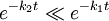 and
and  . Therefore it is valid to apply the steady state approximation only if the second reaction is much faster than the first one (k2/k1 > 10 is a right criterion), because that means that the intermediate forms slowly and reacts readily so its concentration stays low.
 . From then on the concentration of B decreases.


