To use all functions of this page, please activate cookies in your browser.
My watch list
my.chemeurope.com
my.chemeurope.com
With an accout for my.chemeurope.com you can always see everything at a glance – and you can configure your own website and individual newsletter.
- My watch list
- My saved searches
- My saved topics
- My newsletter
Stream functionThe stream function is defined for two-dimensional flows of various kinds. The stream function can be used to plot stream lines, which are perpendicular to equipotential lines. In most cases, the stream function is the imaginary part of the complex potential, while the potential function is the real part. Considering the particular case of fluid dynamics, the difference between the stream function values at any two points gives the volumetric flow rate (or flux) through a line connecting the two points. Note that since streamlines are tangent to the flow, the value of the stream function must be the same along a streamline. If there were a flux across a line, it would necessarily not be tangent to the flow, hence would not be a streamline. The usefulness of the stream function lies in the fact that the velocity components in the x- and y- directions at a given point are given by the partial derivatives of the stream function at that point. A stream function may be defined for any flow of dimensions greater than two, however the two dimensional case is generally the easiest to visualize and derive. Taken together with the velocity potential, the stream function may be used to derive a complex potential for a fluid flow. Product highlight
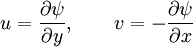
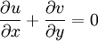
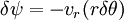
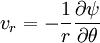
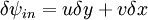
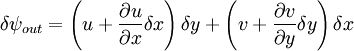
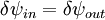
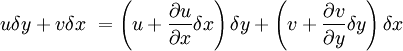
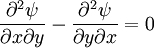
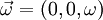
Two dimensional stream functionThe stream function ψ for a two dimensional flow is defined such that the flow velocity can be expressed as: Where In Cartesian coordinate system this is equivalent to Where u and v are the velocities in the This formulation of the stream function satisfies the two dimensional continuity equation: Derivation of the two dimensional stream functionConsider two points A and B in two dimensional plane flow. If the distance between these two points is very small: δn, and a stream of flow passes between these points with an average velocity, q perpendicular to the line AB, the volume flow rate per unit thickness, δΨ is given by: As δn → 0, rearranging this expression, we get: Now consider two dimensional plane flow with reference to a coordinate system. Suppose an observer looks along an arbitrary axis in the direction of increase and sees flow crossing the axis from right to left. A sign convention is adopted such that the velocity of the flow is positive. However, this sign convention is not universal and thus ought to be taken with caution. A couple of examples ought to clarify this point: Flow in Cartesian coordinatesBy observing the flow into an elemental square in an x-y Cartesian coordinate system, we have: where u is the velocity parallel to and in the direction of the x-axis, and v is the velocity parallel to and in the direction of the y-axis. In this case, we have a negative velocity of -u since the flow crosses the y-axis from left to right. Thus as δn → 0 and by rearranging, we have: Flow in Polar coordinatesBy observing the flow into an elemental square in an r-θ Polar coordinate system, we have: where vr is the velocity parallel to and in the direction of the r-axis, and vθ is the velocity parallel to and in the direction of the θ-axis. In this case, we have a negative velocity of -vr since the flow crosses the θ-axis from left to right. Thus as δn → 0 and by rearranging, we have: Continuity: The DerivationConsider two dimensional plane flow within a Cartesian coordinate system. Continuity states that if we consider flow into an elemental square, the flow into that small element must equal the flow out of that element. The total flow into the element is given by: The total flow out of the element is given by: Thus we have: and simplifying to: (NB: Whilst we have ignored the earlier sign convention for Ψ, the mathematics ought work out fine but this proof is perhaps slightly tidier and easier to follow). Substituting the expressions of the stream function into this equation, we have: VorticityIn Cartesian coordinates, the stream function can be found from vorticity using Poisson's equation: where See alsoReferences
Categories: Fluid dynamics | Fluid mechanics |
|
| This article is licensed under the GNU Free Documentation License. It uses material from the Wikipedia article "Stream_function". A list of authors is available in Wikipedia. |


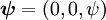 if the velocity vector
 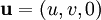 .
.
 and
and  directions, respectively.


 and
and 
Last viewed


