Gas in a box

In quantum mechanics, the results of the quantum particle in a box can be used to look at the equilibrium situation for a quantum ideal gas in a box which is a box containing a large number of molecules which do not interact with each other except for instantaneous thermalizing collisions. This simple model can be used to describe the classical ideal gas as well as the various quantum ideal gases such as the ideal massive Fermi gas, the ideal massive Bose gas as well as black body radiation which may be treated as a massless Bose gas.

Using the results from either Maxwell-Boltzmann statistics, Bose-Einstein statistics or Fermi-Dirac statistics we use the Thomas-Fermi approximation and go to the limit of a very large box, and express the degeneracy of the energy states as a differential, and summations over states as integrals. We will then be in a position to calculate the thermodynamic properties of the gas using the partition function or the grand partition function. These results will be carried out for both massive and massless particles. More complete calculations will be left to separate articles, but some simple examples will be given in this article.

Additional recommended knowledge

How to quickly check pipettes?

Correct Test Weight Handling Guide: 12 Practical Tips

What is the Correct Way to Check Repeatability in Balances?

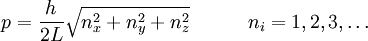
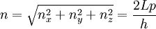
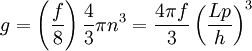
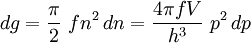
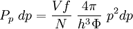
Thomas-Fermi approximation for the degeneracy of states

For both massive and massless particles in a box, the states of a particle are enumerated by a set of quantum numbers. [n_x, n_y, n_z]. The absolute value of the momentum is given by:

where h is Planck's constant and L is the length of a side of the box. We can think of each possible state of a particle as a point on a 3-dimensional grid of positive integers. The distance from the origin to any point will be

Suppose each set of quantum numbers specify f  states where f  is the number of internal degrees of freedom of the particle that can be altered by collision. For example, a spin 1/2 particle would have f=2, one for each spin state. The Thomas-Fermi approximation assumes that the quantum numbers are so large that they may be considered to be a continuum. For large values of n , we can estimate the number of states with absolute value of momentum less than or equal to p from the above equation as

which is just f  times the volume of a sphere of radius n  divided by eight since we only consider the octant with positive n_i . The number of states with absolute value of momentum between p  and p+dp  is therefore

where V=L³  is the volume of the box. Notice that in using this continuum approximation, we have lost the ability to characterize the low-energy states including the ground state where n_i =1. For most cases this will not be a problem, but when considering Bose-Einstein condensation, in which a large portion of the gas is in or near the ground state, we will need to recover the ability to deal with low energy states.

Without using the continuum approximation, the number of particles with energy ε_i is given by

where

	for particles obeying Maxwell-Boltzmann statistics
	for particles obeying Bose-Einstein statistics
	for particles obeying Fermi-Dirac statistics

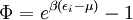
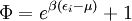
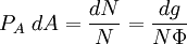
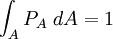
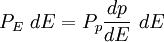
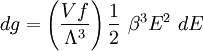
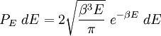
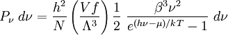
with β = 1/kT  with k  being Boltzmann's constant, T  being temperature, g_i is the degeneracy of the state i, and μ being the chemical potential. Using the continuum approximation, the number of particles dN  with energy between E  and E+dE  is now written:

The energy distribution function

We are now in a position to determine some distribution functions for the "gas in a box". The distribution function for any variable A is P_AdA and is equal to the fraction of particles which have values for A  between A  and A+dA

It follows that:

The distribution function for the absolute value of the momentum is:

and the distribution function for the energy E  is:

For a particle in a box (and for a free particle as well), the relationship between energy E  and momentum p  is different for massive and massless particles. For massive particles, we have

while for massless particles:

where m  is the mass of the particle and c  is the speed of light. Using these relationships we have:

• For massive particles

  

  

  where Λ is the thermal wavelength or thermal de Broglie wavelength of the gas.

  

  This is an important quantity, since when Λ is on the order of the interparticle distance (V/N)^1/3 , quantum effects begin to dominate and the gas can no longer be considered to be a Maxwell-Boltzmann gas. See configuration integral for a detailed derivation of the expression for .
• For massless particles

  

  

  where Λ is now the thermal wavelength for massless particles.

  

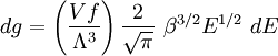
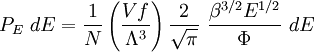
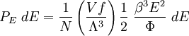
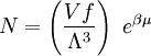
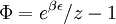
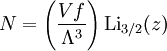
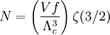
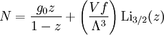
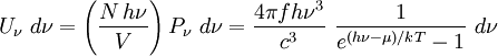
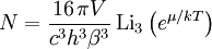
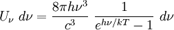
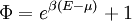
Specific examples

The following sections give an example of results for some specific cases.

Massive Maxwell-Boltzmann particles

For this case:

Integrating the energy distribution function and solving for N gives

Substituting into the original energy distribution function gives

which are the same results obtained classically for the Maxwell-Boltzmann distribution. Further results can be found in the article on the classical ideal gas.

Massive Bose-Einstein particles

For this case:

where z is defined as

Integrating the energy distribution function and solving for N gives the particle number

Where Li_s(z) is the polylogarithm function and Λ is the thermal wavelength. The polylogarithm term must always be positive and real, which means its value will go from 0 to ζ(3/2) as z  goes from 0 to 1. As the temperature drops towards zero, Λ will become larger and larger, until finally Λ will reach a critical value Λ_c where z=1 and

The temperature at which Λ=Λ_c is the critical temperature. For temperatures below this critical temperature, the above equation for the particle number has no solution. The critical temperature is the temperature at which a Bose-Einstein condensate begins to form. The problem is, as mentioned above, that the ground state has been ignored in the continuum approximation. It turns out, however, that the above equation for particle number expresses the number of bosons in excited states rather well, and so we may write:

where the added term is the number of particles in the ground state. (The ground state energy has been ignored.) This equation will hold down to zero temperature. Further results can be found in the article on the ideal Bose gas.

Massless Bose-Einstein particles (e.g. black body radiation)

For the case of massless particles, we must now use the massless energy distribution function. It is convenient to convert this function to a frequency distribution function:

where Λ is the thermal wavelength for massless particles. The spectral energy density (energy per unit volume per unit frequency) is then

Other thermodynamic parameters may be derived analogously to the case for massive particles. For example, integrating the frequency distribution function and solving for N gives the number of particles:

The most common massless Bose gas is a photon gas in a black body. Taking the "box" to be a black body cavity, the photons are continually being absorbed and re-emitted by the walls. When this is the case, the number of photons is not conserved. In the derivation of Bose-Einstein statistics, when the restraint on the number of particles is removed, this is effectively the same as setting the chemical potential (μ) to zero. Furthermore, since photons have two spin states, we have f=2. The spectral energy density is then

which is just the spectral energy density for Planck's law of black body radiation. Note that if we had carried out this procedure for massless Maxwell-Boltzmann particles, we would recover Wien's distribution which approximates a Planck's distribution for high temperature or low density.

In certain situations, the reactions involving photons will result in the conservation of the number of photons (e.g. light-emitting diodes, "white" cavities). In these cases, the photon distribution function will involve a non-zero chemical potential. (Hermann 2005)

Another massless Bose gas is given by the Debye model for heat capacity. This considers a gas of phonons in a box and differs from the development for photons in that the speed of the phonons is less than light speed, and there is a maximum allowed wavelength for each axis of the box. This means that the integration over phase space cannot be carried out to infinity, and instead of results being expressed in polylogarithms, they are expressed in the related Debye functions.

Massive Fermi-Dirac particles (e.g. electrons in a metal)

For this case:

Integrating the energy distribution function gives

Where again, Li_s(z) is the polylogarithm function and Λ is the thermal de Broglie wavelength. Further results can be found in the article on the ideal Fermi gas.

References

• Herrmann, F.; Würfel, P. (August 2005). "Light with nonzero chemical potential". American Journal of Physics 73 (8): 717-723. doi:10.1119/1.1904623. Retrieved on 2006-11-20.
• Huang, Kerson (1967). Statistical Mechanics. New York: John Wiley & Sons. 
• Isihara, A. (1971). Statistical Physics. New York: Academic Press. 
• Landau, L. D.; E. M. Lifshitz (1996). Statistical Physics, 3rd Edition Part 1, Oxford: Butterworth-Heinemann. 
• Yan, Zijun (2000). "General thermal wavelength and its applications" (PDF). Eur. J. Phys. 21: 625-631. doi:10.1088/0143-0807/21/6/314. Retrieved on 2006-11-20.