My watch list

Home
Encyclopedia
Maximum_entropy_probability_distribution

Maximum entropy probability distribution

In statistics and information theory, a maximum entropy probability distribution is a probability distribution whose entropy is at least as great as that of all other members of a specified class of distributions.

If nothing is known about a distribution except that it belongs to a certain class, then the maximum entropy distribution for that class is often chosen as a default, according to the principle of maximum entropy. The motivation is twofold: first, maximizing entropy, in a sense, means minimizing the amount of prior information built into the distribution; second, many physical systems tend to move towards maximal entropy configurations over time.

Additional recommended knowledge

Daily Visual Balance Check

Recognize and detect the effects of electrostatic charges on your balance

Guide to balance cleaning: 8 simple steps

1 Definition of entropy
2 Examples of maximum entropy distributions
3 A theorem by Boltzmann
4 References

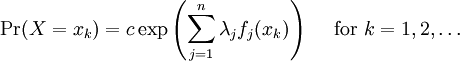
Definition of entropy

If X is a discrete random variable with distribution given by

$\operatorname{Pr}(X=x_k) = p_k \quad\mbox{ for } k=1,2,\ldots$

then the entropy of X is defined as

$H(X) = \sum_{k\ge 1}p_k\log\left({1\over p_k}\right).$

If X is a continuous random variable with probability density p(x), then the entropy of X is defined as

$H(X) = \int_{-\infty}^\infty p(x)\log\left({1\over p(x)}\right) dx$

where p(x) log(1/p(x)) is understood to be zero whenever p(x) = 0.

The base of the logarithm is not important as long as the same one is used consistently: change of base merely results in a rescaling of the entropy. Information theoreticians may prefer to use base 2 in order to express the entropy in bits; mathematicians and physicists will often prefer the natural logarithm, resulting in a unit of nats or nepers for the entropy.

Examples of maximum entropy distributions

Given mean and standard deviation: the normal distribution

The normal distribution N(μ,σ²) has maximum entropy among all real-valued distributions with specified mean μ and standard deviation σ. Therefore, if all you know about a distribution is its mean and standard deviation, it is often reasonable to assume that the distribution is normal.

Uniform and piecewise uniform distributions

The uniform distribution on the interval [a,b] is the maximum entropy distribution among all continuous distributions which are supported in the interval [a, b] (which means that the probability density is 0 outside of the interval).

More generally, if we're given a subdivision a=a₀ < a₁ < ... < a_k = b of the interval [a,b] and probabilities p₁,...,p_k which add up to one, then we can consider the class of all continuous distributions such that

$\operatorname{Pr}(a_{j-1}\le X < a_j) = p_j \quad \mbox{ for } j=1,\ldots,k$

The density of the maximum entropy distribution for this class is constant on each of the intervals [a_j-1,a_j); it looks somewhat like a histogram.

The uniform distribution on the finite set {x₁,...,x_n} (which assigns a probability of 1/n to each of these values) is the maximum entropy distribution among all discrete distributions supported on this set.

Positive and given mean: the exponential distribution

The exponential distribution with mean 1/λ is the maximum entropy distribution among all continuous distributions supported in [0,∞) that have a mean of 1/λ.

In physics, this occurs when gravity acts on a gas that is kept at constant pressure and temperature: if X describes the height of a molecule, then the variable X is exponentially distributed (which also means that the density of the gas depends on height proportional to the exponential distribution). The reason: X is clearly positive and its mean, which corresponds to the average potential energy, is fixed. Over time, the system will attain its maximum entropy configuration, according to the second law of thermodynamics.

Discrete distributions with given mean

Among all the discrete distributions supported on the set {x₁,...,x_n} with mean μ, the maximum entropy distribution has the following shape:

$\operatorname{Pr}(X=x_k) = Cr^{x_k} \quad\mbox{ for } k=1,\ldots, n$

where the positive constants C and r can be determined by the requirements that the sum of all the probabilities must be 1 and the expected value must be μ.

For example, if a large number N of dice is thrown, and you are told that the sum of all the shown numbers is S. Based on this information alone, what would be a reasonable assumption for the number of dice showing 1, 2, ..., 6? This is an instance of the situation considered above, with {x₁,...,x₆} = {1,...,6} and μ = S/N.

Finally, among all the discrete distributions supported on the infinite set {x₁,x₂,...} with mean μ, the maximum entropy distribution has the shape:

$\operatorname{Pr}(X=x_k) = Cr^{x_k} \quad\mbox{ for } k=1,2,\ldots$

where again the constants C and r can be determined by the requirements that the sum of all the probabilities must be 1 and the expected value must be μ.

A theorem by Boltzmann

All the above examples are consequences of the following theorem by Boltzmann.

Continuous version

Suppose S is a closed subset of the real numbers R and we're given n measurable functions f₁,...,f_n and n numbers a₁,...,a_n. We consider the class C of all continuous random variables which are supported on S (i.e. whose density function is zero outside of S) and which satisfy the n expected value conditions

$\operatorname{E}(f_j(X)) = a_j\quad\mbox{ for } j=1,\ldots,n$

If there is a member in C whose density function is positive everywhere in S, and if there exists a maximal entropy distribution for C, then its probability density p(x) has the following shape:

$p(x)=c \exp\left(\sum_{j=1}^n \lambda_j f_j(x)\right)\quad \mbox{ for all } x\in S$

where the constants c and λ_j have to be determined so that the integral of p(x) over S is 1 and the above conditions for the expected values are satisfied.

Conversely, if constants c and λ_j like this can be found, then p(x) is indeed the density of the (unique) maximum entropy distribution for our class C.

This theorem is proved with the calculus of variations and Lagrange multipliers.

Discrete version

Suppose S = {x₁,x₂,...} is a (finite or infinite) discrete subset of the reals and we're given n functions f₁,...,f_n and n numbers a₁,...,a_n. We consider the class C of all discrete random variables X which are supported on S and which satisfy the n conditions

$\operatorname{E}(f_j(X)) = a_j\quad\mbox{ for } j=1,\ldots,n$

If there exists a member of C which assigns positive probability to all members of S and if there exists a maximum entropy distribution for C, then this distribution has the following shape:

$\operatorname{Pr}(X=x_k)=c \exp\left(\sum_{j=1}^n \lambda_j f_j(x_k)\right)\quad \mbox{ for } k=1,2,\ldots$

where the constants c and λ_j have to be determined so that the sum of the probabilities is 1 and the above conditions for the expected values are satisfied.

Conversely, if constants c and λ_j like this can be found, then the above distribution is indeed the maximum entropy distribution for our class C.

This version of the theorem can be proved with the tools of ordinary calculus and Lagrange multipliers.

Caveats

Note that not all classes of distributions contain a maximum entropy distribution. It is possible that a class contain distributions of arbitrarily large entropy (e.g. the class of all continuous distributions on R with mean 0), or that the entropies are bounded above but there is no distribution which attains the maximal entropy (e.g. the class of all continuous distributions X on R with E(X) = 0 and E(X²) = E(X³) = 1).

It is also possible that the expected value restrictions for the class C force the probability distribution to be zero in certain subsets of S. In that case our theorem doesn't apply, but one can work around this by shrinking the set S.

References

T. M. Cover and J. A. Thomas, Elements of Information Theory, 1991. Chapter 11.

v • d • e Probability distributions
	Univariate	Multivariate
Discrete:	Benford · Bernoulli · binomial · Boltzmann · categorical · compound Poisson · discrete phase-type · degenerate · Gauss-Kuzmin · geometric · hypergeometric · logarithmic · negative binomial · parabolic fractal · Poisson · Rademacher · Skellam · uniform · Yule-Simon · zeta · Zipf · Zipf-Mandelbrot	Ewens · multinomial · multivariate Polya
Continuous:	Beta · Beta prime · Cauchy · chi-square · Dirac delta function · Coxian · Erlang · exponential · exponential power · F · fading · Fermi-Dirac · Fisher's z · Fisher-Tippett · Gamma · generalized extreme value · generalized hyperbolic · generalized inverse Gaussian · Half-logistic · Hotelling's T-square · hyperbolic secant · hyper-exponential · hypoexponential · inverse chi-square (scaled inverse chi-square) · inverse Gaussian · inverse gamma (scaled inverse gamma) · Kumaraswamy · Landau · Laplace · Lévy · Lévy skew alpha-stable · logistic · log-normal · Maxwell-Boltzmann · Maxwell speed · Nakagami · normal (Gaussian) · normal-gamma · normal inverse Gaussian · Pareto · Pearson · phase-type · polar · raised cosine · Rayleigh · relativistic Breit-Wigner · Rice · shifted Gompertz · Student's t · triangular · truncated normal · type-1 Gumbel · type-2 Gumbel · uniform · Variance-Gamma · Voigt · von Mises · Weibull · Wigner semicircle · Wilks' lambda	Dirichlet · Generalized Dirichlet · inverse-Wishart · Kent · matrix normal · multivariate normal · multivariate Student · von Mises-Fisher · Wigner quasi · Wishart
Miscellaneous:	bimodal · Cantor · conditional · equilibrium · exponential family · Infinite divisibility (probability) · location-scale family · marginal · maximum entropy · posterior · prior · quasi · sampling · singular · unimodal

Categories: Entropy and information | Particle statistics

This article is licensed under the GNU Free Documentation License. It uses material from the Wikipedia article "Maximum_entropy_probability_distribution". A list of authors is available in Wikipedia.