To use all functions of this page, please activate cookies in your browser.
My watch list
my.chemeurope.com
my.chemeurope.com
With an accout for my.chemeurope.com you can always see everything at a glance – and you can configure your own website and individual newsletter.
- My watch list
- My saved searches
- My saved topics
- My newsletter
Microcanonical ensemble
The microcanonical ensemble is the simplest of the ensembles of statistical mechanics. Additional recommended knowledge
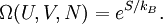
Assumptions of the ensembleA statistical mechanical "ensemble" is a theoretical tool used for analyzing a system. The "ensemble" consists of copies of the system of interest with regards to the fixed and known thermodynamic variables. For example, the microcanonical system is a thermodynamically isolated system, the fixed and known variables are the number of particles in the system, N, the volume of the system, V, and the energy of the system. Therefore, the microcanonical ensemble consists of a set of M systems each characterized by N, V, and E. Each system within the ensemble may be in a different microscopic (quantum) state (i.e. microstate), however, each system shares the same specified thermodynamic properties, here N, V, and E. By the fundamental assumption of thermodynamics, each microstate corresponding to the same energy is equally probable. Therefore, each system within the ensemble is equally probably.
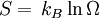
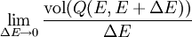
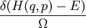
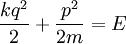
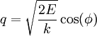
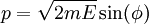
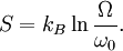
Therefore if Ω is the number of accessible microstates, the probability that a system chosen at random from the ensemble would be in a given microstate is simply The benefit of the ensemble is that it allows for calculation of average values for thermodynamic properties. For example, the pressure of a container of gas fluctuates continuously, however, we measure the pressure as a time average. The ensemble examines all microstates which the system might inhabit during the period of measurement, and determines the probability of each microstate given the thermodynamic properties of the system. Thus, a time average can be obtained as the system will dwell in each microstate probabilistically. A microcanonical ensemble is a degenerate canonical ensemble in the sense that a canonical ensemble can be divided into sub-ensembles, each of which corresponds to a possible energy value and is itself a microcanonical ensemble. Thermodynamical systems that appear in physics are however sometimes constituted of extended objects, eg strings, and in this case the canonical and microcanonical ensembles are not equivalent. One must then resort to the microcanonical ensemble which is thought to be more fundamental. This in turn actually leads to a limiting maximum temperature called the Hagedorn temperature in string theory which has generated a lot of interest and is possibly relevant in the early universe which was, according to observations, much denser and hotter than it is today. We should emphasize that one can calculate with the canonical ensemble but to actually derive a physical quantity, such as the entropy or energy density, one need do so from the microcanonical ensemble, from Ω. (For more information see Deo et al.) EntropyEntropy is defined by where kB is the Boltzmann constant. Or, equivalently, where Ω is the multiplicity of microstates in the ensemble, as before. Notice that, for the microcanonical ensemble, Ω plays the role of the partition function in the canonical and grand canonical ensembles. For this reason, it is also sometimes referred to as the microcanonical partition function. We should note here that the notion of multiplicity Ω is also called the characteristic state function of the microcanonical ensemble. An application: residual entropyThe expression for entropy above can be used to calculate the residual entropy. The third law of thermodynamics says that the entropy of a pure crystalline substance at 0 K is zero. However, in some solids, at temperatures close to 0 K, there may be many molecular orientations. For example, water molecules in ice crystal may arrange themselves in several different ways. In principle, there must be one molecular orientation with the lowest energy. But due the near randomness with which configurations occur, it is often impractical to attempt realization of the lowest energy configuration. This leads to the notion of residual entropy. Furthermore, there are often very little difference in the total energy of the system between the different molecular configurations. Therefore, as an approximation, the system can be viewed having fixed energy and the possible configurations as microstates, exactly a microcanonical ensemble. So it is sensible to estimate the residual entropy via the same expression for the microcanonical ensemble entropy): where Ω is the number of possible molecular arrangements of the crystal, at some suitable temperature range close to 0 K. Classical mechanical systemsAs with any ensemble of classical systems, we would like to find a corresponding probability measure on the phase space M. This constant energy assumption means that every system in the ensemble is confined to a submanifold of phase space of constant energy E. Call this submanifold ME. From the physical considerations given above, it is already clear what the probability measure on the constant energy surface (not the full phase space) should be, namely the trivial one that is constant everywhere. However, while only the submanifold ME is of interest for the microcanonical ensemble, in other more general ensembles, it is necessary to consider the full phase space. We now construct a measure on the full phase space that is suitable for the microcanonical ensemble. The Liouville measure dqdp on the full phase space induces a measure dA on ME in the following manner: The measure of an open subset R of ME is given by Where Q is any open subset of M such that Q ∩ M = R, Q(E, E + ΔE) is part of Q with E < H < E + ΔE, and "vol" is the usual Liouville volume. Thus any sufficiently good (measurable) subset of ME can be characterized by its hyperarea(measure) with respect to dA. The density function on the full phase space ρ(q,p) is the generalized function where ΔE is the intersection of ME and Δ. Notice how one can either consider the whole phase space and use the measure whose density is a generalized function, or restrict to the constant energy surface in question and use the measure whose density is a constant function. For instance, consider a 1-dimensional harmonic oscillator. The phase space is The later can be parametrized as where φ varies between 0 and 2π. The measure dA would then equal dφ up to a constant. On the other hand, if one considers the ellipse embedded in the plane, then it would have measure zero, which is why a generalized function is used as the density. Connection with Liouville's theoremWe have (the curly bracket is Poisson bracket) since ρ is a function of H. Therefore, according to Liouville's theorem we get
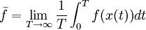
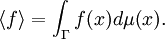
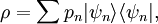
In particular, dA is time-invariant, that is, the ensemble is a stationary one. Alternatively, one can say that since the Liouville measure is invariant under the Hamiltonian flow, so is the measure dA. Physically speaking, this means the local density of a region of representative points in phase space is invariant, as viewed by an observer moving along with the systems. Ergodic hypothesisA microcanonical ensemble of classical systems provides a natural setting to consider the ergodic hypothesis, that is, the long time average coincides with the ensemble average. More precisely put, an observable is a real valued function f on the phase space Γ that is integrable with respect to the microcanonical ensemble measure μ. Let x(0) denote a representative point in the phase space, and x(t) be its image under the Hamiltonian flow at time t. The time average of f is defined to be , provided that this limit exists μ-almost everywhere. The ensemble average is The system is said to be ergodic if they are equal. Using the fact that μ is preserved by the Hamiltonian flow, we can show that indeed the time average exists for all observables. Whether classical mechanical flows on constant energy surfaces is in general ergodic is unknow at this time. RemarkThe relationship between the microcanonical ensemble, Liouville's theorem, and ergodic hypothesis can be summarized as follows: The key assumption of a microcanonial ensemble is that all accessible microstates are equally probable. Therefore the density function on the relevant region of phase space is constant, say it is 1 everywhere, i.e. the phase space measure μ is just the Lebesgue measure. But, according to Liouville's theorem, this measure is invariant under the Hamiltonian time evolution. From this follows that the notion of time average makes sense for all observables. The ensemble average is defined using μ. The question of ergodicity is whether they coincide. It should perhaps be emphasized that while the microcanonical ensemble and Liouville's theorem are directly related, they should not be confused as being equivalent to the ergodic hypothesis. Quantum mechanical systemsSemi-classical treatmentSo far, we have assumed the system in question is classical. Slight modification is required for quantum mechanical systems, although the results are essentially the same. For an ensemble consisting of quantum mechanical systems, it no longer make sense to speak of all members of the ensemble having the same definite energy E. So, instead of a level set H(q,p) = E in the phase space, one considers a small range of energies E < H < E + dE that a system in the ensemble may have and the corresponding region of the phase space. When classical states are replaced by quantum states, the degeneracy needs to be taken into account. Also, in the quantum mechanical case, due to the uncertainty principle, the states can no longer be viewed as continuously distributed in the phase space. Rather, one must find a "fundamental volume" ω0, which depends on the particulars of a given system. As we would expect, ω0 is usually related to Density operatorsThe microcanonical ensemble can also be described by a density operator. Namely, if Ω is the total number of accessible microstates of the system, and where We note here that, in this context, Ω is computed quantum-mechanically, taking into account indistinguishability of particles. The entropy is When Ω = 1, the ensemble is said to be a pure ensemble. The fact that the entropy vanishes for pure states is essentially the third law of thermodynamics. References
|
||||||||
| This article is licensed under the GNU Free Documentation License. It uses material from the Wikipedia article "Microcanonical_ensemble". A list of authors is available in Wikipedia. |


 . This leads to a formula for entropy (see below).
 is valid for any thermodynamical system. Same can be said for partition functions and any ensemble. It is only for the microcanonical ensemble that they happen to be the same.
 , where H is the Hamiltonian and
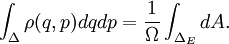
 (the position-momentum plane) and the constant energy hypersurface is the ellipse

 .
.
 in some way. Consequently, the multiplicity is not the total available volume of the phase space
  , and entropy becomes
 are all states of the system (accessible and otherwise), then a microcanonical ensemble is the mixed state
 if
if 

