To use all functions of this page, please activate cookies in your browser.
My watch list
my.chemeurope.com
my.chemeurope.com
With an accout for my.chemeurope.com you can always see everything at a glance – and you can configure your own website and individual newsletter.
- My watch list
- My saved searches
- My saved topics
- My newsletter
Fluctuation theoremThe fluctuation theorem (FT) is a theorem from statistical mechanics dealing with the relative probability that the entropy of a system which is currently away from thermodynamic equilibrium (maximum entropy) will increase or decrease over a given amount of time. The second law of thermodynamics predicts that the entropy of an isolated system should tend to increase until it reaches equilibrium, but after the discovery of statistical mechanics physicists realized that the second law is only a statistical one, so that there should always be some nonzero probability that the entropy of an isolated system will spontaneously decrease; the fluctuation theorem precisely quantifies this probability. Product highlight
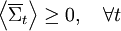
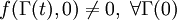
Statement of the fluctuation theorem (roughly)The fluctuation theorem is a statement concerning the probability distribution of the time-averaged irreversible entropy production [1], denoted Mathematically, the FT is expressed as: This means that as the time or system size increases (since Σ is extensive), the probability of observing an entropy production opposite to that dictated by the second law of thermodynamics decreases exponentially. The FT is one of the few expressions in non-equilibrium statistical mechanics that is valid far from equilibrium. The FT was first proposed and tested using computer simulations, by Denis Evans, E.G.D. Cohen and Gary Morriss in 1993 in the journal Physical Review Letters. The first mathematical proof was given by Evans and Debra Searles in 1994. Since then, much mathematical and computational work has been done to show that the FT applies to a variety of statistical ensembles. The first laboratory experiment that verified the validity of the FT was carried out in 2002. In this experiment, a plastic bead was pulled through a solution by a laser. Fluctuations in the velocity were recorded that were opposite to what the second law of thermodynamics would dictate for macroscopic systems. See Wang et al. [Phys Rev Lett, 89, 050601(2002)] and later Carberry et al, [Phys Rev Lett, 92, 140601(2004)]. This work was widely reported in the press - Second law of thermodynamics "broken" (NewScientist, 19 July 2002); Nature July 23, 2002, http://www.nature.com/nsu/020722/020722-2.html . Note that the FT does not state that the second law of thermodynamics is wrong or invalid. The second law of thermodynamics is a statement about macroscopic systems. The FT is more general. It can be applied to both microscopic and macroscopic systems. When applied to macroscopic systems, the FT is equivalent to the Second Law of Thermodynamics. Second law inequalityA simple consequence of the fluctuation theorem given above is that if we carry out an ensemble of experiments from some initial time t=0, and perform an ensemble average of time averages of the entropy production then an exact consequence of the FT is that the ensemble average cannot be negative for any value of the averaging time t: For rather obvious reasons this equality is called the Second Law Inequality [Searles & Evans, Aust J Chem, 57, 1119 (2004)]. This inequality can be proved for systems with time dependent fields of arbitrary magnitude and arbitrary time dependence. It is important to understand what the Second Law Inequality does not imply. It does not imply that the ensemble averaged entropy production is non-negative at all times. This is clearly untrue as consideration of the entropy production in a viscoelastic fluid subject to a sinusoidal time dependent shear rate clearly shows. In this example the ensemble average of the time integral of the entropy production is however non negative - as expected from the Second Law Inequality. Nonequilibrium partition identityAnother remarkably simple and elegant consequence of the FT is the so-called "nonequilibrium partition identity" (NPI): see Carberry et al J Chem Phys 121, 8179(2004). Thus in spite of the Second Law Inequality which might lead you to expect that the average would decay exponentially with time, the exponential probability ratio given by the FT exactly cancels the negative exponential in the average above leading to an average which is unity for all time! There are many important implications from the FT. One is that small machines (such as nanomachines or even mitochondria in a cell) will spend part of their time actually running in "reverse". By "reverse", it is meant that they function so as to run in a way opposite to that for which they were presumably designed. As an example, consider a jet engine. If a jet engine were to run in "reverse" in this context, it would take in ambient heat and exhaust fumes to generate kerosene and oxygen. Dissipation function[1] Strictly speaking the fluctuation theorem refers to a quantity known as the dissipation function. In thermostatted nonequilibrium states that are close to equilibrium, the long time average of the dissipation function is equal to the average entropy production. However the FT refers to fluctuations rather than averages. The dissipation function is defined as, where k is Boltzmann's constant, f(Γ,0) is the initial (t = 0) distribution of molecular states Γ, and Γ(t) is the molecular state arrived at after time t, under the exact time reversible equations of motion. f(Γ(t),0) is the INITIAL distribution of those time evolved states. Note: in order for the FT to be valid we require that The system may be in contact with a large heat reservoir in order to thermostat the system of interest. If this is the case ΔQ(t) is the heat lost to the reservoir over the time (0,t) and T is the absolute equilibrium temperature of the reservoir - see Williams et al, Phys Rev E70, 066113(2004). With this definition of the dissipation function the precise statement of the FT simply replaces entropy production with the dissipation function in each of the FT equations above. Example: If one considers electrical conduction across an electrical resistor in contact with a large heat reservoir at temperature T, then the dissipation function is
the total electric current density J multiplied by the voltage drop across the circuit, Fe, and the system volume V, divided by the absolute temperature T, of the heat reservoir times Boltzmann's constant. Thus the dissipation function is easily recognised as the Ohmic work done on the system divided by the temperature of the reservoir. Close to equilibrium the long time average of this quantity is (to leading order in the voltage drop), equal to the average spontaneous entropy production per unit time - see de Groot and Mazur "Nonequilibrium Thermodynamics" (Dover), equation (61), page 348. However, the Fluctuation Theorem applies to systems arbitrariliy far from equilibrium where the definition of the spontaneous entropy production is problematic. The fluctuation theorem and Loschmidt's paradoxThe second law of thermodynamics, which predicts that the entropy of an isolated system out of equilibrium should tend to increase rather than decrease or stay constant, stands in apparent contradiction with the time-reversible equations of motion for classical and quantum systems, which tell us that for any physical process that is compatible with these fundamental laws, a second process that looked exactly like a film of the first process played backward would also be compatible with these same fundamental laws, and would in fact be equally likely if the initial state was picked at random from the phase space of all possible states for the system. This is often referred to as Loschmidt's paradox. The FT is sometimes argued to provide a resolution to this paradox since its derivation assumes time-reversible laws, but it does not really solve the problem. Although the FT does predict the entropy of a system in a nonequilibrium state is more likely to have increased at a later time than it is to have decreased, the FT is still time-symmetric in the sense that one could use the same derivation to "retrodict" earlier states of a system currently in a nonequilibrium state, and the FT would work the same way in reverse, predicting that the system was more likely to have been at higher entropy at earlier times rather than lower entropy.[citation needed] This second prediction would be frequently violated in films of nonequilibrium systems played backwards, since it is often true that such a system was at an even lower entropy in the past (although the prediction would be correct if the nonequilibrium state were the result of a random fluctuation in entropy in an isolated system that had previously been at equilibrium - in this case, if you happen to observe the system in a lower-entropy state, it is most likely that you are seeing the minimum of the random dip in entropy, in which case entropy would be higher on either side of this minimum). So, it seems that the asymmetry that is at the heart of Loschmidt's paradox has still not been explained. Most modern physicists believe the answer to Loschmidt's paradox lies in the smooth low-entropy state of the universe shortly after the big bang, although the explanation for this state itself is still debated.[citation needed] SummaryThe fluctuation theorem is of fundamental importance to nonequilibrium statistical mechanics. The FT (together with the Axiom of Causality) gives a generalisation of the second law of thermodynamics which includes as a special case, the conventional second law. It is then easy to prove the Second Law Inequality and the NonEquilibrium Partition Identity. When combined with the central limit theorem, the FT also implies the famous Green-Kubo relations for linear transport coefficients, close to equilibrium. The FT is however, more general than the Green-Kubo Relations because unlike them, the FT applies to fluctuations far from equilibrium. In spite of this fact, scientists have not yet been able to derive the equations for nonlinear response theory from the FT. The FT does not imply or require that the distribution of time averaged dissipation be Gaussian. There are many examples known where the distribution of time averaged dissipation is non-Gaussian and yet the FT (of course) still correctly describes the probability ratios. Lastly the theoretical constructs used to prove the FT can been applied to nonequilibrium transitions between two different equilibrium states. When this is done the so-called Jarzynski equality or nonequilibrium work relation, can be derived. This equality shows how equilibrium free energy differences can be computed or measured (in the laboratory), from nonequilibrium path integrals. Previously quasi-static (equilibrium) paths were required. The reason why the fluctuation theorem is so fundamental is that its proof requires so little. It requires:
In regard to the latter "assumption", all the equations of motion for either classical or quantum dynamics are in fact time reversible. References
See also
Categories: Statistical mechanics | Non-equilibrium thermodynamics |
|
| This article is licensed under the GNU Free Documentation License. It uses material from the Wikipedia article "Fluctuation_theorem". A list of authors is available in Wikipedia. |


 . The theorem states that, in systems away from equilibrium over a finite time t, the ratio between the probability that
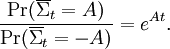
![\left\langle {\exp [ - \overline \Sigma_t \; t ]} \right\rangle = 1,\quad \forall t](images/math/6/6/1/66166cf20c6c15652bef6b9003342353.png)
![\Omega _t (\Gamma ) = \int_0^t {ds\;\Omega (\Gamma ;s)} \equiv \ln \left[ {\frac{{f(\Gamma ,0)}}{{f(\Gamma (t),0)}}} \right] - \frac{{\Delta Q(\Gamma ;t)}}{kT}](images/math/d/9/f/d9f9c1d6972f794596bd7c3f8cdd0ff8.png)
 . This condition is known as the condition of ergodic consistency. It is widely satisfied in common
 Last viewed


