To use all functions of this page, please activate cookies in your browser.
My watch list
my.chemeurope.com
my.chemeurope.com
With an accout for my.chemeurope.com you can always see everything at a glance – and you can configure your own website and individual newsletter.
- My watch list
- My saved searches
- My saved topics
- My newsletter
Radiative transfer equation and diffusion theory for photon transport in biological tissuePhoton transport in biological tissue can be equivalently modeled numerically with Monte Carlo simulations or analytically by the radiative transfer equation (RTE). However, the RTE is difficult to solve without introducing approximations. A common approximation summarized here is the diffusion approximation. Overall, solutions to the diffusion equation for photon transport are more computationally efficient, but less accurate than Monte Carlo simulations[1]. Product highlight
Definitions
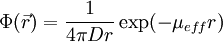
The RTE can mathematically model the transfer of energy as photons move inside a tissue. The flow of radiation energy through a small area element in the radiation field can be characterized by radiance
Radiative transfer equationThe RTE is a differential equation describing radiance where
Diffusion theoryAssumptionsIn the RTE, six different independent variables define the radiance at any spatial and temporal point (x, y, and z from
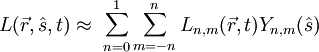
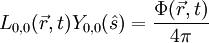
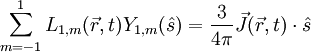
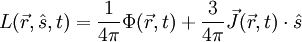
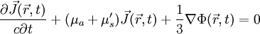
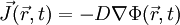
It should be noted that both of these assumptions require a high-albedo (predominantly scattering) medium[1]. The RTE in the diffusion approximationRadiance can be expanded on a basis set of spherical harmonics Yn,m. In diffusion theory, radiance is taken to be largely isotropic, so only the isotropic and first-order anisotropic terms are used: where Ln,m are the expansion coefficients. Radiance is expressed with 4 terms; one for n = 0 (the isotropic term) and 3 terms for n = 1 (the anisotropic terms). Using properties of spherical harmonics and the definitions of fluence rate Hence we can approximate radiance as[1] Substituting the above expression for radiance, the RTE can be respectively rewritten in scalar and vector forms as follows (The scattering term of the RTE is integrated over the complete 4π solid angle. For the vector form, the RTE is multiplied by direction The diffusion equationUsing the second assumption of diffusion theory, we note that the fractional change in current density
Solutions to the diffusion equationFor various configurations of boundaries (eg layers of tissue) and light sources, the diffusion equation may be solved by applying appropriate boundary conditions and defining the source term Point sources in infinite homogeneous mediaA solution to the diffusion equation for the simple case of a short-pulsed point source in an infinite homogeneous medium is presented in this section. The source term in the diffusion equation becomes The term
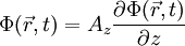
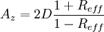
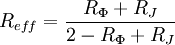
Boundary conditionsFluence rate at a boundaryConsideration of boundary conditions permits use of the diffusion equation to characterize light propagation in media of limited size (where interfaces between the medium and the ambient environment must be considered). To begin to address a boundary, one can consider what happens when photons in the medium reach a boundary (ie a surface). The direction-integrated radiance at the boundary and directed into the medium is equal to the direction-integrated radiance at the boundary and directed out of the medium multiplied by reflectance RF: where Substituting Fick's law ( The extrapolated boundaryIt is desirable to identify a zero-fluence boundary. However, the fluence rate Φ(z = 0,t) at a physical boundary is, in general, not zero. An extrapolated boundary, at zb for which fluence rate is zero, can be determined to establish image sources. Using a first order Taylor series approximation, which evaluates to zero since Pencil beam normally incident on a semi-infinite mediumUsing boundary conditions, one may approximately characterize diffuse reflectance for a pencil beam normally incident on a semi-infinite medium. The beam will be represented as two point sources in an infinite medium as follows (Figure 2)[1][3]:
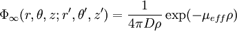
The two point sources can be characterized as point sources in an infinite medium via ρ is the distance from observation point (r,θ,z) to source location (r',θ',z') in cylindrical coordinates. The linear combination of the fluence rate contributions from the two image sources is This can be used to get diffuse reflectance Rd(r) via Fick's law:
Diffusion theory solutions vs. Monte Carlo simulationsMonte Carlo simulations of photon transport, though time consuming, will accurately predict photon behavior in a scattering medium. The assumptions involved in characterizing photon behavior with the diffusion equation generate inaccuracies. Generally, the diffusion approximation is less accurate as the absorption coefficient μa increases and the scattering coefficient μs decreases. For a photon beam incident on a medium of limited depth, error due to the diffusion approximation is most prominent within one transport mean free path of the location of photon incidence (where radiance is not yet isotropic) (Figure 3).
See also
Further reading
References
Categories: Electromagnetic radiation | Light |
|
| This article is licensed under the GNU Free Documentation License. It uses material from the Wikipedia article "Radiative_transfer_equation_and_diffusion_theory_for_photon_transport_in_biological_tissue". A list of authors is available in Wikipedia. |
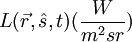 . Radiance is defined as energy flow per unit normal area per unit solid angle per unit time. Here,
  denotes position,
  denotes unit direction vector and
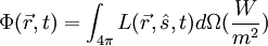
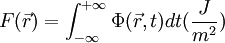
 . This is the vector counterpart of fluence rate pointing in the prevalent direction of energy flow.
 . It can be derived via
 is the phase function, representing the probability of light with propagation direction
  being scattered into solid angle
 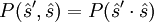 . The scattering anisotropy can be expressed as
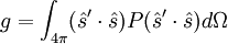
 describes the light source.
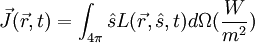
 and current density
  , the isotropic and anisotropic terms can respectively be expressed as follows:
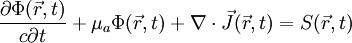
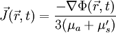 , which defines current density in terms of the gradient of fluence rate. Substituting Fick's law into the scalar representation of the RTE gives the diffusion equation
![\frac{\partial \Phi(\vec{r},t)}{c\partial t} + \mu_a\Phi(\vec{r},t) + \nabla \cdot [D\nabla\Phi(\vec{r},t)] = S(\vec{r},t)](images/math/3/7/8/3784717628b76c18413afac71451db72.png)
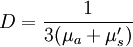 is the diffusion coefficient and μ's
 as the situation demands.
 , where
  is the position of the source. The pulse peaks at time
 ![\Phi(\vec{r},t;\vec{r'},t)=\frac{c}{[4\pi Dc(t-t')^{3/2}]}\exp\left[-\frac{\mid \vec{r}-\vec{r'} \mid ^2}{rDc(t-t')}\right]\exp[-\mu_ac(t-t')]](images/math/d/5/d/d5df21f4253e387c798185a8b28cc68c.png)
![\exp\left[-\mu_ac(t-t')\right]](images/math/6/f/d/6fd68ca6da626e2b1262d75182cc2c94.png) represents the exponential decay in fluence rate due to absorption in accordance with
represents the exponential decay in fluence rate due to absorption in accordance with  :
:
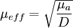 is the effective attenuation coefficient and indicates the rate of spatial decay in fluence
 is normal to and pointing away from the boundary. The diffusion approximation gives an expression for radiance
  . Evaluating the above integrals after substitution gives
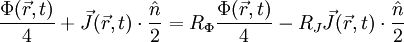
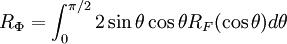
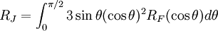
 ) gives, at a distance from the boundary z=0