To use all functions of this page, please activate cookies in your browser.
My watch list
my.chemeurope.com
my.chemeurope.com
With an accout for my.chemeurope.com you can always see everything at a glance – and you can configure your own website and individual newsletter.
- My watch list
- My saved searches
- My saved topics
- My newsletter
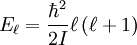
Rigid rotorThe rigid rotor is a mechanical model that is used to explain rotating systems. An arbitrary rigid rotor is a 3-dimensional rigid object, such as a top. To orient such an object in space three angles are required. A special rigid rotor is the linear rotor which is a 2-dimensional object, requiring two angles to describe its orientation. An example of a linear rotor is a diatomic molecule. More general molecules like water (asymmetric rotor), ammonia (symmetric rotor), or methane (spherical rotor) are 3-dimensional, see classification of molecules. Product highlight
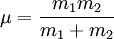
The linear rotorThe linear rigid rotor model consists of two point masses located at fixed distances from their center of mass. The fixed distance between the two masses and the values of the masses are the only characteristics of the rigid model. However, for many actual diatomics this model is too restrictive since distances are usually not completely fixed. Corrections on the rigid model can be made to compensate for small variations in the distance. Even in such a case the rigid rotor model is a useful point of departure (zeroth-order model). The classical linear rigid rotorThe classical linear rotor consists of two point masses m1 and m2
(with reduced mass where Scale factors are of importance for quantum mechanical applications since they enter the Laplacian expressed in curvilinear coordinates. In the case at hand (constant R) The classical Hamiltonian function of the linear rigid rotor is The quantum mechanical linear rigid rotorThe linear rigid rotor model can be used in quantum mechanics to predict the rotational energy of a diatomic molecule. The rotational energy depends on the moment of inertia for the system, I. In the center of mass reference frame, the moment of inertia is equal to:
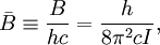
where μ is the reduced mass of the molecule and R is the distance between the two atoms. According to quantum mechanics, the energy levels of a system can be determined by solving the Schrödinger equation: where Y is the wave function and where This operator appears also in the Schrödinger equation of the hydrogen atom after the radial part is separated off. The eigenvalue equation becomes The symbol is Introducing the rotational constant B, we write, In the unit of reciprocal length the rotational constant is, with c the speed of light. If cgs units are used for h, c, and I, A typical rotational spectrum consists of a series of peaks that correspond to transitions between levels with different values of the angular momentum quantum number ( Selection rulesRotational transitions of a molecule occur when the molecule absorbs a photon [a particle of a quantized electromagnetic (em) field]. Depending on the energy of the photon (i.e., the wavelength of the em field) this transition may be seen as a sideband of a vibrational and/or electronic transition. Pure rotational transitions, in which the vibronic (= vibrational plus electronic) wave function does not change, occur in the microwave region of the em spectrum. Typically, rotational transitions can only be observed when the angular momentum quantum number changes by 1 ( A transition occurs if this integral is non-zero. By separating the rotational part of the molecular wavefunction from the vibronic part, one can show that this means that the molecule must have a permanent dipole moment. After integration over the vibronic coordinates the following rotational part of the transition moment remains, Here Non-rigid linear rotorThe rigid rotor is commonly used to describe the rotational energy of diatomic molecules but it is not a completely accurate description of such molecules. This is because molecular bonds (and therefore the interatomic distance R) are not completely fixed; the bond between the atoms stretches out as the molecule rotates faster (higher values of the rotational quantum number l). This effect can be accounted for by introducing a correction factor known as the centrifugal distortion constant where
The non-rigid rotor is an acceptably accurate model for diatomic molecules but is still somewhat imperfect. This is because, although the model does account for bond stretching due to rotation, it ignores any bond stretching due to vibrational energy in the bond (anharmonicity in the potential). Arbitrarily shaped rigid rotorAn arbitrarily shaped rigid rotor is a rigid body of arbitrary shape with its center of mass fixed (or in uniform rectilinear motion) in field-free space R3, so that its energy consists only of rotational kinetic energy (and possibly constant translational energy that can be ignored). A rigid body can be (partially) characterized by the three eigenvalues of its moment of inertia tensor, which are real nonnegative values known as principal moments of inertia. In microwave spectroscopy—the spectroscopy based on rotational transitions—one usually classifies molecules (seen as rigid rotors) as follows:
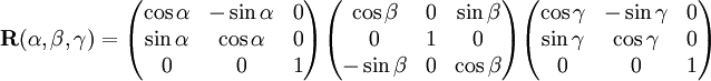
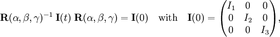
This classification depends on the relative magnitudes of the principal moments of inertia. Coordinates of the rigid rotorDifferent branches of physics and engineering use different coordinates for the description of the kinematics of a rigid rotor. In molecular physics Euler angles are used almost exclusively. In quantum mechanical applications it is advantageous to use Euler angles in a convention that is a simple extension of the physical convention of spherical polar coordinates. The first step is the attachment of a right-handed orthonormal frame (3-dimensional system of orthogonal axes) to the rotor (a body-fixed frame) . This frame can be attached arbitrarily to the body, but often one uses the principal axes frame—the normalized eigenvectors of the inertia tensor, which always can be chosen orthonormal, since the tensor is symmetric. When the rotor possesses a symmetry-axis, it usually coincides with one of the principal axes. It is convenient to choose as body-fixed z-axis the highest-order symmetry axis. One starts by aligning the body-fixed frame with a space-fixed frame
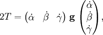
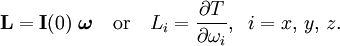
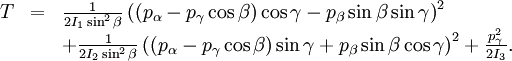
(laboratory axes), so that the body-fixed x, y, and z axes coincide with the space-fixed X, Y, and Z axis. Secondly, the body and its frame are rotated actively over a positive angle If the body lacks cylinder (axial) symmetry, a last rotation around its z-axis (which has polar coordinates The convention for Euler angles described here is known as the z'' − y' − z convention; it can be shown (in the same manner as in this article) that it is equivalent to the z − y − z convention in which the order of rotations is reversed. The total matrix of the three consecutive rotations is the product Let In particular, if which shows the correspondence with the spherical polar coordinates (in the physical convention). Knowledge of the Euler angles as function of time t and the initial coordinates Classical kinetic energyThe following text forms a generalization of the well-known special case of the rotational energy of an object that rotates around one axis. It will be assumed from here on that the body-fixed frame is a principal axes frame; it diagonalizes the instantaneous inertia tensor where the Euler angles are time-dependent and in fact determine the time dependence of The classical kinetic energy T of the rigid rotor can be expressed in different ways:
Since each of these forms has its use and can be found in textbooks we will present all of them. Angular velocity formAs a function of angular velocity T reads, with The vector Lagrange formBacksubstitution of the expression of where Angular momentum formOften the kinetic energy is written as a function of the angular momentum Since the body-fixed frame moves (depends on time) these components are not time independent. If we were
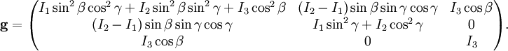
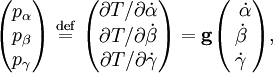
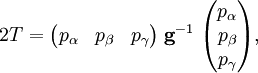
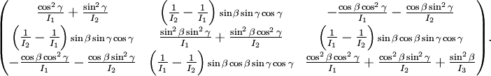
to represent Hamilton formThe Hamilton form of the kinetic energy is written in terms of generalized momenta where it is used that the with the inverse metric tensor given by This inverse tensor is needed to obtain the Laplace-Beltrami operator, which (multiplied
by The classical Hamiltonian given above can be rewritten to the following expression, which is needed in the phase integral arising in the classical statistical mechanics of rigid rotors, Quantum mechanical rigid rotorAs usual quantization is performed by the replacement of the generalized momenta by operators that give first derivatives with respect to its canonically conjugate variables (positions). Thus, and similarly for pβ and pγ. It is remarkable that this rule replaces the fairly complicated function pα of all three Euler angles, time derivatives of Euler angles, and inertia moments (characterizing the rigid rotor) by a simple differential operator that does not depend on time or inertia moments and differentiates to one Euler angle only. The quantization rule is sufficient to obtain the operators
that correspond with the classical angular momenta. There are two kinds: space-fixed and body-fixed
angular momentum operators. Both are vector operators, i.e., both have three components
that transform as vector components among themselves upon rotation of the space-fixed and the body-fixed frame, respectively. The explicit form of the rigid rotor angular momentum operators is
given here (but beware, they must be multiplied with The quantization rule is not sufficient to obtain the kinetic energy operator from
the classical Hamiltonian. Since classically pβ commutes with cosβ and sinβ and the inverses of these functions, the position
of these trigonometric functions in the classical Hamiltonian is arbitrary. After
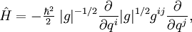
quantization the commutation does no longer hold and the order of operators and functions in the Hamiltonian (energy operator) becomes a point of concern. Podolsky[1] proposed in 1928 that the Laplace-Beltrami operator
(times where | g | is the determinant of the g-tensor: Given the inverse of the metric tensor above, the explicit form of the kinetic energy operator in terms of Euler angles follows by simple substitution. The corresponding eigenvalue equation gives the Schrödinger equation for the rigid rotor in the form that it was solved for the first time by Kronig and Rabi[2] (for the special case of the symmetric rotor). This is one of the few cases where the Schrödinger equation can be solved analytically. All these cases were solved within a year of the formulation of the Schrödinger equation. Nowadays it is common to proceed as follows. It can be shown that The action of the so that the Schrödinger equation for the spherical rotor (I = I1 = I2 = I3)
is solved with the (2j + 1)2 degenerate energy equal to The symmetric top (= symmetric rotor) is characterized by I1 = I2. It is a prolate (cigar shaped) top if I3 < I1 = I2. In the latter case we write the Hamiltonian as and use that Hence The eigenvalue Ej0 is 2j + 1-fold degenerate, for all eigenfunctions
with The asymmetric top problem ( ReferencesCited references General references
See also |
|
| This article is licensed under the GNU Free Documentation License. It uses material from the Wikipedia article "Rigid_rotor". A list of authors is available in Wikipedia. |


 ) at a distance
  , the longitudinal (azimuth) angle
  and the distance
 ![2T = \mu R^2\big [\dot{\theta}^2+(\dot\varphi\,\sin\theta)^2\big]= \mu R^2 \big(\dot{\theta}\;\; \dot{\varphi} \Big) \begin{pmatrix} 1 & 0 \\ 0 & \sin^2 \theta \\ \end{pmatrix} \begin{pmatrix} \dot{\theta}\\ \dot{\varphi} \end{pmatrix} = \mu \Big(\dot{\theta}\;\; \dot{\varphi} \Big) \begin{pmatrix} h_\theta^2 & 0 \\ 0 & h_\varphi^2 \\ \end{pmatrix} \begin{pmatrix} \dot{\theta}\\ \dot{\varphi} \end{pmatrix},](images/math/0/b/9/0b95acaf64dd6cae2f0cf2e38dd9a9ed.png)
 and
and 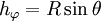 are
scale (or Lamé) factors.
are
scale (or Lamé) factors.
![\nabla^2 = \frac{1}{h_\theta h_\varphi}\left[ \frac{\partial}{\partial \theta} \frac{h_\varphi}{h_\theta} \frac{\partial}{\partial \theta} +\frac{\partial}{\partial \varphi} \frac{h_\theta}{h_\varphi} \frac{\partial}{\partial \varphi} \right]= \frac{1}{R^2}\left[\frac{1}{\sin\theta} \frac{\partial}{\partial \theta} \sin\theta \frac{\partial}{\partial \theta} +\frac{1}{\sin^2\theta}\frac{\partial^2}{\partial \varphi^2} \right].](images/math/f/f/5/ff54584fae92d1e5e76c4aa797d306ac.png)
![H = \frac{1}{2\mu R^2}\left[p^2_{\theta} + \frac{p^2_{\varphi}}{\sin^2\theta}\right].](images/math/d/c/4/dc4f5760ed7424d599c8e167dcae4708.png)

 is the energy (Hamiltonian) operator. For the rigid rotor in a field-free space, the energy operator corresponds to the kinetic energy
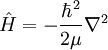
 is Planck's constant divided by
  is the Laplacian. The Laplacian is given above in terms of spherical polar coordinates. The energy operator written in terms of these coordinates is:
![\hat H =- \frac{\hbar^2}{2I} \left [ {1 \over \sin \theta} {\partial \over \partial \theta} \left ( \sin \theta {\partial \over \partial \theta} \right ) + {1 \over {\sin^2 \theta}} {\partial^2 \over \partial \varphi^2} \right]](images/math/b/e/8/be8462f5e7ae2ea6a44eb9712a08ee87.png)
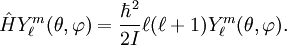
 represents a set of functions known as the
  . The energy
 -fold degenerate: the functions with fixed
  and
and 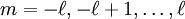 have the same energy.

 is expressed
in wave numbers, cm-1, a unit that is often used for rotational-vibrational spectroscopy.
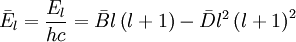
The rotational constant
is expressed
in wave numbers, cm-1, a unit that is often used for rotational-vibrational spectroscopy.
The rotational constant  depends on the distance
  where
where  ). Consequently,
  .
.
 ). This selection rule arises from a first-order perturbation theory approximation of the time-dependent Schrödinger equation. According to this treatment, rotational transitions can only be observed when one or more
components of the
). This selection rule arises from a first-order perturbation theory approximation of the time-dependent Schrödinger equation. According to this treatment, rotational transitions can only be observed when one or more
components of the 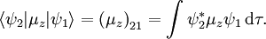

 is the z component of the permanent dipole moment. The moment
  it is possible to determine which values of
 (bars on top of various quantities indicate that these quantities are expressed in cm-1):

 is the fundamental vibrational frequency of the bond (in cm-1). This frequency is related to the reduced mass and the
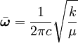
 around the z-axis (by the right-hand rule), which moves the
  around the
  .
.
 be the coordinate vector of an arbitrary point
  in the body with respect to the body-fixed frame. The elements of
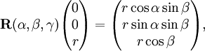
 (expressed with respect to the space-fixed frame), i.e.,
![T = \frac{1}{2} \left[ I_1 \omega_x^2 + I_2 \omega_y^2+ I_3 \omega_z^2 \right]](images/math/1/5/6/1567e4fb259766941584a80d25480f84.png)
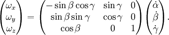
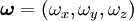 contains the components of the angular velocity of the rotor expressed with respect to the body-fixed frame. It can be shown that
  is not the time derivative of any vector, in contrast to the usual definition of velocity. The dots over the time-dependent Euler angles indicate time derivatives.
The angular velocity satisfies equations of motion known as Euler's equations (with zero applied torque, since by assumption the rotor is in field-free space).
is not the time derivative of any vector, in contrast to the usual definition of velocity. The dots over the time-dependent Euler angles indicate time derivatives.
The angular velocity satisfies equations of motion known as Euler's equations (with zero applied torque, since by assumption the rotor is in field-free space).
 is the metric tensor expressed in Euler angles—a non-orthogonal system of curvilinear coordinates—
 of the rigid rotor. This vector is a conserved (time-independent) quantity.
With respect to the body-fixed frame it has the components
of the rigid rotor. This vector is a conserved (time-independent) quantity.
With respect to the body-fixed frame it has the components  , which can be shown to
be related to the angular velocity,
, which can be shown to
be related to the angular velocity,
![T = \frac{1}{2} \left[ \frac{L_x^2}{I_1} + \frac{L_y^2}{I_2}+ \frac{L_z^2}{I_3}\right].](images/math/4/a/c/4ac24bebd7c5e648a6763fb6c2d6f6e5.png)

 ) gives the quantum mechanical energy operator
of the rigid rotor.
) gives the quantum mechanical energy operator
of the rigid rotor.
 . They satisfy anomalous commutation relations.
 ) has the appropriate form for the quantum mechanical kinetic
energy operator. This operator has the general form (summation convention: sum over repeated indices—in this case over the three Euler angles
) has the appropriate form for the quantum mechanical kinetic
energy operator. This operator has the general form (summation convention: sum over repeated indices—in this case over the three Euler angles  ):
):

 can be expressed in body-fixed angular momentum operators (in this proof one must carefully
commute differential operators with trigonometric functions). The result has the same appearance
as the classical formula expressed in body-fixed coordinates,
can be expressed in body-fixed angular momentum operators (in this proof one must carefully
commute differential operators with trigonometric functions). The result has the same appearance
as the classical formula expressed in body-fixed coordinates,
![\hat{H} = \tfrac{1}{2}\left[ \frac{\mathcal{P}_x^2}{I_1}+ \frac{\mathcal{P}_y^2}{I_2}+ \frac{\mathcal{P}_z^2}{I_3} \right].](images/math/e/c/7/ec73bc0a45a9dd954eea9a5917e10bbb.png)

 .
.
![\hat{H} = \tfrac{1}{2}\left[ \frac{\mathcal{P}^2}{I_1}+ \mathcal{P}_z^2\Big(\frac{1}{I_3} -\frac{1}{I_1} \Big) \right],](images/math/d/c/8/dc81bcf96fa8ab7774408255881d49a7.png)


 have the same eigenvalue. The energies with |k| > 0 are
 ) is not exactly soluble.


