My watch list

Home
Encyclopedia
Boussinesq_approximation_(water_waves)

Boussinesq approximation (water waves)

In fluid dynamics, the Boussinesq approximation for water waves is an approximation valid for weakly non-linear and fairly long waves. The approximation is named after Joseph Boussinesq, who first derived them in response to the observation of the solitary wave made by John Scott Russell. The 1872 paper of Boussinesq, for the first time introducing the equations now known as the Boussinesq equations, starts with:

"Touts les ingénieurs connaisants les belles expériences de J. Scott Russell and M. Basin sur la production et la propagation des ondes solitaires."

The Boussinesq approximation for water waves takes into account the vertical structure of the horizontal and vertical flow velocity. This results in non-linear partial differential equations, called Boussinesq-type equations, which incorporate frequency dispersion (as opposite to the shallow water equations, which are not frequency-dispersive).

In coastal engineering, Boussinesq-type equations are frequently used in computer models for the simulation of water waves in shallow seas and harbours.

Additional recommended knowledge

Weighing the right way

Daily Visual Balance Check

Daily Sensitivity Test

1 Boussinesq approximation
2 Original Boussinesq equations
3 Extensions
4 Further approximations for one-way wave propagation
5 References

Boussinesq approximation

The essential idea in the Boussinesq approximation is the eliminatation of the vertical coordinate from the flow equations, while retaining some of the influences of the vertical structure of the flow under water waves. This was first done by Joseph Boussinesq in 1871 to construct an approximate solution for the solitary wave (or wave of translation), and subsequently in 1872 to derive the equations now known as the Boussinesq equations.

The steps in the Boussinesq approximation are:

a Taylor expansion is made of the horizontal and vertical flow velocity (or velocity potential) around a certain elevation,
this Taylor expansion is truncated to a finite number of terms,
the continuity equation for an incompressible flow and the zero-curl condition for an irrotational flow are used, to replace vertical partial derivatives of quantities in the Taylor expansion with horizontal partial derivatives.

Thereafter, the Boussinesq approximation is applied to the remaining flow equations, in order to eliminate the dependence on the vertical coordinate. As a result, the resulting partial differential equations are in terms of functions of the horizontal coordinates (and time).

As an example, consider potential flow over a horizontal bed in the (x,z) plane, with x the horizontal and z the vertical coordinate. The bed is located at z=0, around which level we make a Taylor expansion of the velocity potential φ(x,z,t):

$\phi = \phi_b + z \left[ \frac{\partial \phi}{\partial z } \right]_{z=0} + \frac{1}{2} z^2 \left[ \frac{\partial^2 \phi}{\partial z^2} \right]_{z=0} + \frac{1}{6} z^3 \left[ \frac{\partial^3 \phi}{\partial z^3} \right]_{z=0} + \frac{1}{24} z^4 \left[ \frac{\partial^4 \phi}{\partial z^4} \right]_{z=0} + \cdots,$

where φ_b(x,t) is the velocity potential at the bed. Invoking Laplace's equation for φ, as valid for incompressible flow, we get:

$\begin{align} \phi & = \left\{ \phi_b - \frac{1}{2} z^2 \frac{\partial^2 \phi_b}{\partial x^2} + \frac{1}{24} z^4 \frac{\partial^4 \phi_b}{\partial x^4} + \cdots \right\} \quad + \quad \left\{ z \left[ \frac{\partial \phi}{\partial z} \right]_{z=0} - \frac{1}{6} z^3 \frac{\partial^2}{\partial x^2} \left[ \frac{\partial \phi}{\partial z} \right]_{z=0} + \cdots \right\} \\ & = \left\{ \phi_b - \frac{1}{2} z^2 \frac{\partial^2 \phi_b}{\partial x^2} + \frac{1}{24} z^4 \frac{\partial^4 \phi_b}{\partial x^4} + \cdots \right\}, \end{align}$

since the vertical velocity $\partial \phi/\partial z$ is zero at the horizontal bed z=0. This series may subsequently be truncated to a finite number of terms.

Original Boussinesq equations

For water waves on an incompressible fluid and irrotational flow, the boundary conditions at the free surface elevation z = η(x,t) are:

$\frac{\partial \eta}{\partial t}\, +\, u\, \frac{\partial \eta}{\partial x}\, -\, w\, =\, 0 \quad \text{and} \quad \frac{\partial \phi}{\partial t}\, +\, \frac{1}{2}\, \left( u^2 + w^2 \right)\, +\, g\, \eta\, =\, 0, \quad \text{with} \quad u\, =\, \frac{\partial \phi}{\partial x} \text{ and } w\, =\, \frac{\partial \phi}{\partial z},$

where:

u is the horizontal flow velocity component,

w is the vertical flow velocity component,

g is the acceleration by gravity and

h is the mean water depth.

Now the Boussinesq approximation for the velocity potential φ, as given above, is applied in these boundary conditions. Further, the resulting equations are only allowed to have linear and quadratic terms of η and u_b (the x-derivative of φ_b). Then, the following partial differential equations are obtained:

set A — Boussinesq (1872), equation (25)

$\begin{align} \frac{\partial \eta}{\partial t}\, & +\, \frac{\partial}{\partial x}\, \left[ \left( h + \eta \right)\, u_b \right]\, =\, \frac{1}{6}\, h^3\, \frac{\partial^3 u_b}{\partial x^3}, \\ \frac{\partial u_b}{\partial t}\, & +\, u_b\, \frac{\partial u_b}{\partial x}\, +\, g\, \frac{\partial \eta}{\partial x}\, =\, \frac{1}{2}\, h^2\, \frac{\partial^3 u_b}{\partial t\, \partial^2 x}. \end{align}$

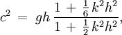
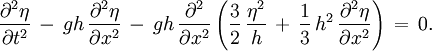
This set of equations has been derived for a flat horizontal bed, i.e. the mean depth h is a constant independent of position x. When the right-hand sides of the above equations are set to zero, they reduce to the shallow water equations.

The linear frequency dispersion characteristics of this set A of equations is:

$c^2\, =\; g h\, \frac{ 1\, +\, \frac{1}{6}\, k^2 h^2 }{ 1\, +\, \frac{1}{2}\, k^2 h^2 },$

with c the phase speed and k the wave number.

Under some additional approximations, the above set A can be reduced to a single partial differential equation for the free surface elevation η:

set B — Boussinesq (1872), equation (26)

$\frac{\partial^2 \eta}{\partial t^2}\, -\, g h\, \frac{\partial^2 \eta}{\partial x^2}\, -\, g h\, \frac{\partial^2}{\partial x^2} \left( \frac{3}{2}\, \frac{\eta^2}{h}\, +\, \frac{1}{3}\, h^2\, \frac{\partial^2 \eta}{\partial x^2} \right)\, =\, 0.$

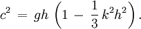
The linear frequency dispersion characteristics of this equation B are:

$c^2\, =\, g h\, \left( 1\, -\, \frac{1}{3}\, k^2 h^2 \right).$

For kh > 1/3 the approximation becomes physically meaningless because there are no longer real-valued solutions. The original set of two partial differential equations (Boussinesq, 1872, equation 25, see set A above) does not have this shortcoming.

Extensions

There is an overwhelming amount of mathematical models which are referred to as Boussinesq equations. This may easily lead to confusion, since often they are loosely referenced to as the Boussinesq equations, while in fact a variant thereof is considered. So it is more appropiate to call them Boussinesq-type equations. Strictly speaking, the Boussinesq equations is the above mentioned set B, since it is used in the analysis in the remainder of his 1872 paper.

Some directions, into which the Boussinesq equations have been extended, are:

varying bathymetry,
improved frequency dispersion,
improved non-linear behavior,
making a Taylor expansion around different vertical elevations,
inclusion of wave breaking,
inclusion of surface tension,
extension to internal waves on an interface between fluid domains of different mass density,
derivation from a variational principle.

Further approximations for one-way wave propagation

While the Boussinesq equations allow for waves traveling in any direction, it is often advantageous to only consider waves traveling in one direction. Under small additional assumptions, the Boussinesq equations reduce to

the Korteweg–de Vries equation for wave propagation in one horizontal dimension,
the Kadomtsev–Petviashvili equation for wave propagation in two horizontal dimensions.

References

J. Boussinesq (1871) Théorie de l'intumescence liquide, applelée onde solitaire ou de translation, se propageant dans un canal rectangulaire, Comptes Rendus de l'Academie des Sciences 72:755–759.
J. Boussinesq (1872) Théorie des ondes et des remous qui se propagent le long d'un canal rectangulaire horizontal, en communiquant au liquide contenu dans ce canal des vitesses sensiblement pareilles de la surface au fond. Journal de Mathématique Pures et Appliquées, Deuxième Série, 17:55–108.
M.W. Dingemans (1997) Wave propagation over uneven bottoms. Advanced Series on Ocean Engineering, Vol. 13, World Scientific, Singapore. See Part 2, Chapter 5.
D.H. Peregrine (1967) Long waves on a beach. Journal of Fluid Mechanics 27(4): 815–827.
D.H. Peregrine (1972) Equations for water waves and the approximations behind them. In Waves on Beaches and Resulting Sediment Transport, Ed. R.E. Meyer, Academic Press: 95–122.

Category: Fluid dynamics

This article is licensed under the GNU Free Documentation License. It uses material from the Wikipedia article "Boussinesq_approximation_(water_waves)". A list of authors is available in Wikipedia.