To use all functions of this page, please activate cookies in your browser.
My watch list
my.chemeurope.com
my.chemeurope.com
With an accout for my.chemeurope.com you can always see everything at a glance – and you can configure your own website and individual newsletter.
- My watch list
- My saved searches
- My saved topics
- My newsletter
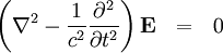
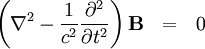
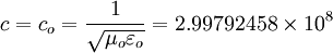
Electromagnetic wave equationThe electromagnetic wave equation is a second-order partial differential equation that describes the propagation of electromagnetic waves through a medium or in a vacuum. The homogeneous form of the equation, written in terms of either the electric field E or the magnetic field B, takes the form: where c is the speed of light in the medium. In a vacuum, c = 299792458 meters per second, which is the speed of light in free space. The electromagnetic wave equation derives from Maxwell's equations. It should also be noted that in most older literature, B is called the "magnetic flux density" or "magnetic induction". Product highlightSpeed of propagationIn vacuumIf the wave propagation is in vacuum, then
is the speed of light in vacuum. The magnetic constant
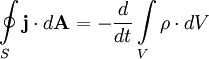
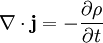
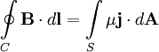
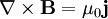
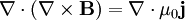
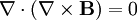
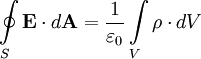
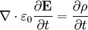
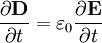
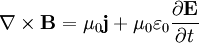
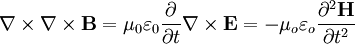
In a material mediumThe speed of light in a linear, isotropic, and non-dispersive material medium is where is the refractive index of the medium, The origin of the electromagnetic wave equationConservation of chargeConservation of charge requires that the time rate of change of the total charge enclosed within a volume V must equal the net current flowing into the surface S enclosing the volume: where j is the current density (in Amperes per square meter) flowing through the surface and ρ is the charge density (in coulombs per cubic meter) at each point in the volume. From the divergence theorem, this relationship can be converted from integral form to differential form: Ampère's circuital law prior to Maxwell's correctionIn its original form, Ampère's circuital law relates the magnetic field B to the current density j: which can be converted to differential form, using Stokes' theorem: Inconsistency between Ampère's circuital law and the law of conservation of chargeTaking the divergence of both sides of Ampère's circuital law gives: The divergence of the curl of any vector field, including the magnetic field B, is always equal to zero: Combining these two equations implies that Because However, the law of conservation of charge tells that Hence, as in the case of Kirchhoff's circuit laws, Ampère's circuital law would appear only to hold in situations involving constant charge density. This would rule out the situation that occurs in the plates of a charging or a discharging capacitor. Maxwell's correction to Ampère's circuital lawGauss's law in integral form states: which can be converted to differential form using the divergence theorem: Taking the time derivative of both sides and reversing the order of differentiation on the left-hand side gives: This last result, along with Ampère's circuital law and the conservation of charge equation, suggests that there are actually two origins of the magnetic field: the current density j, as Ampère had already established, and the so-called displacement current: So the corrected form of Ampère's circuital law becomes: Maxwell's hypothesis that light is an electromagnetic wave
In his 1864 paper entitled A Dynamical Theory of the Electromagnetic Field, Maxwell utilized the correction to Ampère's circuital law that he had made in part III of his 1861 paper On Physical Lines of Force. In PART VI of his 1864 paper which is entitled 'ELECTROMAGNETIC THEORY OF LIGHT'. [1] (page 497 of the article and page 9 of the pdf link) Maxwell combined displacement current with some of the other equations of electromagnetism and he obtained a wave equation with a speed equal to the speed of light. He commented:
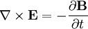
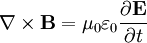
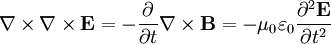
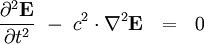
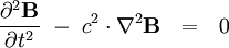
(see [2], page 499 of the article and page 1 of the pdf link) Maxwell's derivation of the electromagnetic wave equation has been replaced in modern physics by a much less cumbersome method involving combining the corrected version of Ampère's circuital law with Faraday's law of induction. To obtain the electromagnetic wave equation in a vacuum using the modern method, we begin with the modern 'Heaviside' form of Maxwell's equations. In a vacuum, these equations are: Taking the curl of the curl equations gives: By using the vector identity where where
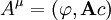
is the speed of light in free space. Covariant form of the homogeneous wave equationThese relativistic equations can be written in covariant form as where the electromagnetic four-potential is with the Lorenz gauge condition:
Here
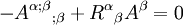
Homogeneous wave equation in curved spacetimeThe electromagnetic wave equation is modified in two ways, the derivative is replaced with the covariant derivative and a new term that depends on the curvature appears. where is the Ricci curvature tensor and the semicolon indicates covariant differentiation. The generalization of the Lorenz gauge condition in curved spacetime is assumed:
Inhomogeneous electromagnetic wave equationLocalized time-varying charge and current densities can act as sources of electromagnetic waves in a vacuum. Maxwell's equations can be written in the form of a wave equation with sources. The addition of sources to the wave equations makes the partial differential equations inhomogeneous. Solutions to the homogeneous electromagnetic wave equationThe general solution to the electromagnetic wave equation is a linear superposition of waves of the form and for virtually any well-behaved function g of dimensionless argument φ, where
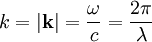
Although the function g can be and often is a monochromatic sine wave, it does not have to be sinusoidal, or even periodic. In practice, g cannot have infinite periodicity because any real electromagnetic wave must always have a finite extent in time and space. As a result, and based on the theory of Fourier decomposition, a real wave must consist of the superposition of an infinite set of sinusoidal frequencies. In addition, for a valid solution, the wave vector and the angular frequency are not independent; they must adhere to the dispersion relation: where k is the wavenumber and λ is the wavelength. Monochromatic, sinusoidal steady-stateThe simplest set of solutions to the wave equation result from assuming sinusoidal waveforms of a single frequency in separable form: where
Plane wave solutionsConsider a plane defined by a unit normal vector
Then planar traveling wave solutions of the wave equations are and where
These solutions represent planar waves traveling in the direction of the normal vector
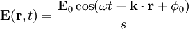
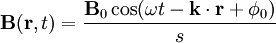
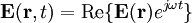
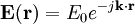
Because the divergence of the electric and magnetic fields are zero, there are no fields in the direction of propagation. This solution is the linearly polarized solution of the wave equations. There are also circularly polarized solutions in which the fields rotate about the normal vector. Spectral decompositionBecause of the linearity of Maxwell's equations in a vacuum, solutions can be decomposed into a superposition of sinusoids. This is the basis for the Fourier transform method for the solution of differential equations. The sinusoidal solution to the electromagnetic wave equation takes the form
and where
The wave vector is related to the angular frequency by where k is the wavenumber and λ is the wavelength. The Electromagnetic spectrum is a plot of the field magnitudes (or energies) as a function of wavelength. Other solutionsSpherically symmetric and cylindrically symmetric analytic solutions to the electromagnetic wave equations are also possible. In cylindrical coordinates the wave equation can be written as follows: and ReferencesElectromagnetismJournal articles
http://www.zpenergy.com/downloads/Maxwell_1864_1.pdf http://www.zpenergy.com/downloads/Maxwell_1864_2.pdf http://www.zpenergy.com/downloads/Maxwell_1864_3.pdf http://www.zpenergy.com/downloads/Maxwell_1864_4.pdf http://www.zpenergy.com/downloads/Maxwell_1864_5.pdf http://www.zpenergy.com/downloads/Maxwell_1864_6.pdf Undergraduate-level textbooks
Graduate-level textbooks
Vector calculus
See alsoTheory and Experiment
Applications
Biographies
|
||||||||||||||||||||||
| This article is licensed under the GNU Free Documentation License. It uses material from the Wikipedia article "Electromagnetic_wave_equation". A list of authors is available in Wikipedia. |


 meters per second
 and the vacuum permittivity
  are important physical constants that play a key role in electromagnetic theory.


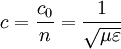

 is the magnetic permeability of the medium, and
  is the electric permittivity of the medium.


 is any vector function of space, it turns into the wave equations:
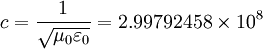 meters per second

 .
.
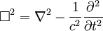 is the d'Alembertian operator. The square box is not a typographical error; it is the correct symbol for this operator.

 .
.


 is the angular frequency (in radians per second), and
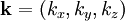 is the wave vector (in radians per meter).
 is the imaginary unit,
 is the angular frequency in
  is the frequency in
 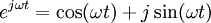 is Euler's formula.
 .
.
 is the position vector (in meters).
 .
If we define the z direction as the direction of
.
If we define the z direction as the direction of  , then by Faraday's Law the magnetic field lies in the y direction and is related to the electric field by the relation
 .
.


 is time (in seconds),
 is the phase angle (in radians).