To use all functions of this page, please activate cookies in your browser.
My watch list
my.chemeurope.com
my.chemeurope.com
With an accout for my.chemeurope.com you can always see everything at a glance – and you can configure your own website and individual newsletter.
- My watch list
- My saved searches
- My saved topics
- My newsletter
Ideal chainAn ideal chain (or freely-jointed chain) is the simplest model to describe a polymer. It only assumes a polymer as a random walk and neglects any kind of interactions among monomers. Although it is simple, its generality gives us some insights about the physics of polymers. In this model, monomers are rigid rods of a fixed length l, and their orientation is completely independent of the orientations and positions of neighbouring monomers, to the extent that two monomers can co-exist at the same place. N monomers form the polymer, whose total unfolded length is:
In this very simple approach where no interactions between monomers are considered, the energy of the polymer is taken to be independent of its shape, which means that at thermodynamic equilibrium, all of its shape configurations are equally likely to occur as the polymer fluctuates in time, according to the Maxwell-Boltzmann distribution. Let us call The two ends of the chain are not coincident, but they fluctuate around each other, so that of course: Throughout the article the Since So that
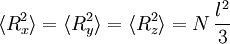
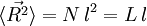
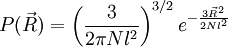
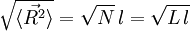
The average end-to-end distance of the polymer is: A quantity frequently used in polymer physics is the radius of gyration: It is worth noting that the above average end-to-end distance, which in the case of this simple model is also the typical amplitude of the system's fluctuations, becomes negligible compared to the total unfolded length of the polymer Mathematical remark: the rigorous demonstration of the expression of the density of probability Product highlight
Generality of the modelWhile the elementary model described above is totally unadapted to the description of real-world polymers at the microscopic scale, it does show some relevance at the macroscopic scale in the case of a polymer in solution whose monomers form an ideal mix with the solvent (in which case, the interactions between monomer and monomer, solvent molecule and solvent molecule, and between monomer and solvent are identical, and the system's energy can be considered constant, validating the hypothesis of the model). The relevancy of the model is, however, limited, even at the macroscopic scale, by the fact that it does not consider any excluded volume for monomers (or, to speak in chemical terms, that it neglects steric effects). Other fluctuating polymer models that consider no interaction between monomers and no excluded volume, like the worm-like chain model, are all asymptotically convergent toward this model at the thermodynamic limit. For purpose of this analogy a Kuhn segment is introduced, corresponding to the equivalent monomer length to be considered in the analogous ideal chain. The number of Kuhn segments to be considered in the analogous ideal chain is equal to the total unfolded length of the polymer divided by the length of a Kuhn segment. Entropic elasticity of an ideal chainIf the two free ends of an ideal chain are attached to some kind of micro-manipulation device, then the device experiences a force exerted by the polymer. The ideal chain's energy is constant, and thus its time-average, the internal energy, is also constant, which means that this force necessarily stems from a purely entropic effect. This entropic force is very similar to the pressure experienced by the walls of a box containing an ideal gas. The internal energy of an ideal gas depends only on its temperature, and not on the volume of its containing box, so it is not an energy effect that tends to increase the volume of the box like gas pressure does. This implies that the pressure of an ideal gas has a purely entropic origin. What is the microscopic origin of such an entropic force or pressure? The most general answer is that the effect of thermal fluctuations tends to bring a thermodynamic system toward a macroscopic state that corresponds to a maximum in the number of microscopic states (or micro-states) that are compatible with this macroscopic state. In other words, thermal fluctuations tend to bring a system toward its macroscopic state of maximum entropy. What does this mean in the case of the ideal chain? First, for our ideal chain, a microscopic state is characterized by the superposition of the states In this section, the mean of this force will be derived. The generality of the expression obtained at the thermodynamic limit will then be discussed. Ideal chain under length constraintThe case of an ideal chain whose two ends are attached to fixed points will be considered in this sub-section. The vector
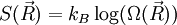
The above expression gives the absolute (quantum) entropy of the system. A precise determination of
where Cst is a fixed constant. Let us call δW is defined as the elementary amount of mechanical work transferred by the operator to the ideal chain, and δQ is defined as the elementary amount of heat transferred by the solvent to the ideal chain. Now, if we assume that the transformation imposed by the operator on the system is quasistatic (i.e., infinitely slow), then the system's transformation will be time-reversible, and we can assume that during its passage from macro-state
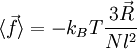
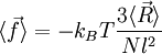
We are thus led to: The above equation is the equation of state of the ideal chain. Since the expression depends on the central limit theorem, it is only exact in the limit of polymers containing a large number of monomers (that is, the thermodynamic limit). Ideal polymer exchanging length with a reservoirThroughout this sub-section, as in the previous one, the two ends of the polymer are attached to a micro-manipulation device. This time, however, the device does not maintain the two ends of the ideal chain in a fixed position, but rather it maintains a constant pulling force For an ideal chain exchanging length with a reservoir, a macro-state of the system is characterized by the vector The change between an ideal chain of fixed length and an ideal chain in contact with a length reservoir is very much akin to the change between the micro-canonical ensemble and the canonical ensemble (see the Statistical mechanics article about this). The change is from a state where a fixed value is imposed on a certain parameter, to a state where the system is left free to exchange this parameter with the outside. The parameter in question is energy for the microcanonical and canonical descriptions, whereas in the case of the ideal chain the parameter is the length of the ideal chain. Like for the micro-canonical and canonical ensembles, the two descriptions of the ideal chain differ only in the way they treat the system's fluctuations. They are thus equivalent at the thermodynamic limit. The equation of state of the ideal chain remains the same, except that
See also
Categories: Polymer chemistry | Polymer physics |
|
| This article is licensed under the GNU Free Documentation License. It uses material from the Wikipedia article "Ideal_chain". A list of authors is available in Wikipedia. |
 , where N is the number of monomers.
 the total end to end vector of an ideal chain and
  the vectors corresponding to individual
 brackets will be used to denote the mean (of values taken over time) of a random variable or a random vector, as above.

 . The end to end vector of the chain is distributed according to the following probability density function:

 at the thermodynamic limit. This result is a general property of statistical systems.
 is not as direct as it appears above: from the application of the usual (1D) central limit theorem one can deduce that
  . Then, the expression given above for


 of each individual monomer (with i varying from 1 to N). In its solvent, the ideal chain is constantly subject to shocks from moving solvent molecules, and each of these shocks sends the system from its current microscopic state to another, very similar microscopic state. For an ideal polymer, as will be shown below, there are more microscopic states compatible with a short end-to-end distance than there are microscopic states compatible with a large end-to-end distance. Thus, for an ideal chain, maximizing its entropy means reducing the distance between its two free ends. Consequently, a force that tends to collapse the chain is exerted by the ideal chain between its two free ends.
 (micro-states are defined in the introduction to this section). Since the ideal chain's energy is constant, each of these micro-states is equally likely to occur. The entropy associated to a macro-state is thus equal to:
 , where
 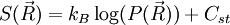 ,
,
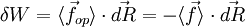
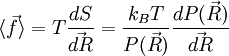
 the force exerted by the chain on the point to which its end is attached. From the above expression of the entropy, we can deduce an expression of this force. Suppose that, instead of being fixed, the positions of the two ends of the ideal chain are now controlled by an operator. The operator controls the evolution of the end to end vector
  , then the variation of
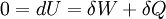
 , the system passes through a series of
  , where T is the temperature of the chain.
 the force exerted by the operator and
  the force exerted by the chain, we have:
 .
.
 .
.


