To use all functions of this page, please activate cookies in your browser.
My watch list
my.chemeurope.com
my.chemeurope.com
With an accout for my.chemeurope.com you can always see everything at a glance – and you can configure your own website and individual newsletter.
- My watch list
- My saved searches
- My saved topics
- My newsletter
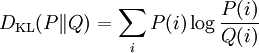
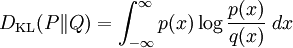
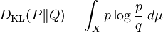
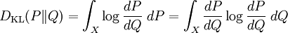
Kullback–Leibler divergenceIn probability theory and information theory, the Kullback–Leibler divergence (also information divergence, information gain, or relative entropy) is a measure of the difference between two probability distributions: from a "true" probability distribution P to an arbitrary probability distribution Q. Although it is often intuited as a distance metric, the KL divergence is not a true metric since it is not symmetric (hence 'divergence' rather than 'distance'). Typically P represents data, observations, or a precise calculated probability distribution. The measure Q typically represents a theory, a model, a description or an approximation of P. For probability distributions P and Q of a discrete random variable the K–L divergence (or informally K–L distance) of Q from P is defined to be For distributions P and Q of a continuous random variable the summations give way to integrals, so that where p and q denote the densities of P and Q. Generalising the two examples above, if dP = pdμ and dQ = qdμ are probability measures over a set X, absolutely continuous with respect to a measure μ then the Kullback-Leibler divergence from P to Q is defined as provided the right hand exists. If P is absolutely continuous with respect to Q,
(which is necessary if
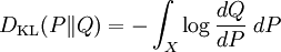
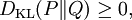
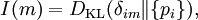
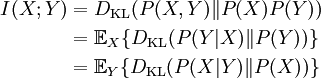
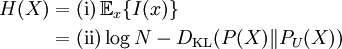
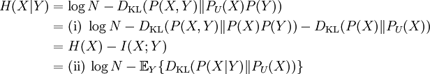
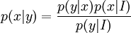
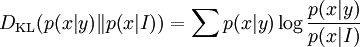
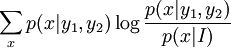
which we recognise as the entropy of P relative to Q. Likewise if Q is absolutely continuous with respect to P then In either case, we see that the Kullback Leibler divergence does not depend on the auxiliary measure μ The logarithms in these formulae are taken to base 2 if information is measured in units of bits, or to base e if information is measured in nats. Most formulas involving the KL divergence hold irrespective of log base. Product highlightMotivation, properties and terminologyIn information theory, the Kraft-McMillan theorem establishes that any directly-decodable coding scheme for coding a message to identify one value xi out of a set of possibilities X can be seen as representing an implicit probability distribution q(xi) = 2-li over X, where li is the length of the code for xi in bits. Therefore, KL divergence can be interpreted as the expected extra message-length per datum that must be communicated if a code that is optimal for a given (wrong) distribution Q is used, compared to using a code based on the true distribution P. It can be seen from the definition of the Kullback-Leibler divergence that where H(P,Q) is called the cross entropy of P and Q, and H(P) is the entropy of P. The Kullback–Leibler divergence is always non-negative, a result known as Gibbs' inequality, with DKL(P||Q) zero if and only if P = Q. The entropy H(P) thus sets a minimum value for the cross-entropy H(P,Q), the expected number of bits required when using a code based on Q rather than P; and the KL divergence therefore represents the expected number of extra bits that must be transmitted to identify a value x drawn from X, if a code is used corresponding to the probability distribution Q, rather than the "true" distribution P. Originally introduced by Solomon Kullback and Richard Leibler in 1951 as the directed divergence between two distributions, it is not the same as a divergence in calculus. One might be tempted to call it a "distance metric" on the space of probability distributions, but this would not be correct as the Kullback-Leibler divergence is not symmetric, Moreover, DKL(P||Q) does not satisfy the triangle inequality. Following Renyi (1961), the term is sometimes also called the information gain about X achieved if P can be used instead of Q. It is also called the relative entropy, for using Q instead of P. The Kullback–Leibler divergence remains well-defined for continuous distributions, and furthermore is invariant under parameter transformations. It can therefore be seen as in some ways a more fundamental quantity than some other properties in information theory (such as self-information or Shannon entropy), which can become undefined or negative for non-discrete probabilities. Relation to other quantities of information theoryMany of the other quantities of information theory can be interpreted as applications of the KL divergence to specific cases. The self-information, is the KL divergence of the probability distribution P(i) from a Kronecker delta representing certainty that i=m — i.e. the number of extra bits that must be transmitted to identify i if only the probability distribution P(i) is available to the receiver, not the fact that i=m. The mutual information, is the KL divergence of the product P(X)P(Y) of the two marginal probability distributions from the joint probability distribution P(X,Y) — i.e. the expected number of extra bits that must be transmitted to identify X and Y if they are coded using only their marginal distributions instead of the joint distribution. Equivalently, if the joint probability P(X,Y) is known, it is the expected number of extra bits that must on average be sent to identify Y if the value of X is not already known to the receiver. The Shannon entropy, is the number of bits which would have to be transmitted to identify X from N equally likely possibilities, less the KL divergence of the uniform distribution PU(X) from the true distribution P(X) — i.e. less the expected number of bits saved, which would have had to be sent if the value of X were coded according to the uniform distribution PU(X) rather than the true distribution P(X). The conditional entropy, is the number of bits which would have to be transmitted to identify X from N equally likely possibilities, less the KL divergence of the product distribution PU(X) P(Y) from the true joint distribution P(X,Y) — i.e. less the expected number of bits saved which would have had to be sent if the value of X were coded according to the uniform distribution PU(X) rather than the conditional distribution P(X|Y) of X given Y. KL divergence and Bayesian updatingIn Bayesian statistics the KL divergence can be used as a measure of the information gain in moving from a prior distribution to a posterior distribution. If some new fact Y=y is discovered, it can be used to update the probability distribution for X from p(x|I) to a new posterior probability distribution p(x|y) using Bayes' theorem: This distribution has a new entropy, H(p(x|y)) = -∑ p(x|y) log p(x|y), which may be less than or greater than the original entropy H(p(x|I)). However, from the standpoint of the new probability distribution one can estimate that to have used the original code based on p(x|I) instead of a new code based on p(x|y) would have added an expected number of bits to the message length. This therefore represents the amount of useful information, or information gain, about X, that we can estimate has been learned by discovering Y=y. If a further piece of data, Y2=y2, subsequently comes in, the probability distribution for x can be updated further, to give a new best guess p(x|y1,y2). If one reinvestigates the information gain for using p(x|y1) rather than p(x|I), it turns out that it may be either greater or less than previously estimated:
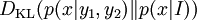
and so the combined information gain does not obey the triangle inequality:
All one can say is that on average, averaging using p(y2|y1,x), the two sides will average out. Bayesian experimental designIn Bayesian experimental design a design which is optimised to maximise the KL divergence between the prior and the posterior is said to be Bayes d-optimal. Discrimination informationThe Kullback–Leibler divergence DKL( p(x|H1) || p(x|H0) ) can also be interpreted as the expected discrimination information for H1 over H0: the mean information per sample for discriminating in favour of a hypothesis H1 against a hypothesis H0, when hypothesis H1 is true. Another name for this quantity, given to it by I.J. Good, is the expected weight of evidence for H1 over H0 to be expected from each sample. The expected weight of evidence for H1 over H0 is not the same as the information gain expected per sample about the probability distribution p(H) of the hypotheses,
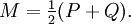
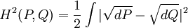
Either of the two quantities can be used as a utility function in Bayesian experimental design, to choose an optimal next question to investigate: but they will in general lead to rather different experimental strategies. On the entropy scale of information gain there is very little difference between near certainty and absolute certainty -- coding according to a near certainty requires hardly any more bits than coding according to an absolute certainty. On the other hand, on the logit scale implied by weight of evidence, the difference between the two is enormous - infinite perhaps; this might reflect the difference between being almost sure (on a probabilistic level) that, say, the Riemann hypothesis is correct, compared to being certain that it is correct because one has a mathematical proof. These two different scales of loss function for uncertainty are both useful, according to how well each reflects the particular circumstances of the problem in question. Principle of minimum discrimination informationThe idea of Kullback–Leibler divergence as discrimination information led Kullback to propose the Principle of Minimum Discrimination Information (MDI): given new facts, a new distribution f should be chosen which is as hard to discriminate from the original distribution f0 as possible; so that the new data produces as small an information gain DKL( f || f0 ) as possible. For example, if one had a prior distribution p(x,a) over x and a, and subsequently learnt the true distribution of a was u(a), the Kullback–Leibler divergence between the new joint distribution for x and a, q(x|a) u(a), and the earlier prior distribution would be: i.e. the sum of the KL divergence of p(a) the prior distribution for a from the updated distribution u(a), plus the expected value (using the probability distribution u(a)) of the KL divergence of the prior conditional distribution p(x|a) from the new conditional distribution q(x|a). This is minimised if q(x|a) = p(x|a) over the whole support of u(a); and we note that this result incorporates Bayes' theorem, if the new distribution u(a) is in fact a δ function representing certainty that a has one particular value. MDI can be seen as an extension of Laplace's Principle of Insufficient Reason, and the Principle of Maximum Entropy of E.T. Jaynes. In particular, it is the natural extension of the principle of maximum entropy from discrete to continuous distributions, for which Shannon entropy ceases to be so useful (see differential entropy), but the KL divergence continues to be just as relevant. In the engineering literature, MDI is sometimes called the Principle of Minimum Cross-Entropy (MCE) or Minxent for short. This is not entirely helpful. Minimising the KL divergence of m from p with respect to m is equivalent to minimising the cross-entropy of p and m, since which is appropriate if one is trying to choose a least 'brain-damaged' approximation to p. However, this is just as often not the task one is trying to achieve. Instead, just as often it is m that is some fixed prior reference measure, and p that one is attempting to optimise by minimising DKL(p||m) subject to some constraint. This has led to some ambiguity in the literature, with some authors attempting to resolve the inconsistency by redefining cross-entropy to be DKL(p||m), rather than H(p,m). Quantum information theoryFor density matrices P and Q on a Hilbert space the K–L divergence (or relative entropy as it is often called in this case) from P to Q is defined to be In quantum information science it can also be used as a measure of entanglement in a state. Symmetrised divergenceKullback and Leibler themselves actually defined the divergence as: which is symmetric and nonnegative. This quantity has sometimes been used for feature selection in classification problems, where P and Q are the conditional pdfs of a feature under two different classes. An alternative is given via the λ divergence, which can be interpreted as the expected information gain about X from discovering which probability distribution X is drawn from, P or Q, if they currently have probabilities λ and (1 − λ) respectively. The value λ = 0.5 gives the Jensen-Shannon divergence, defined by where M is the average of the two distributions, DJS can also be interpreted as the capacity of a noisy information channel with two inputs giving the output distributions p and q. The Jensen-Shannon divergence is the square of a metric that is equivalent to the Hellinger metric, and the Jensen-Shannon divergence is also equal to one-half the so-called Jeffreys divergence (Rubner et al., 2000; Jeffreys 1946). Relationship to Hellinger DistanceIf P and Q are two probability measures, then the squared Hellinger distance is the quantity given by
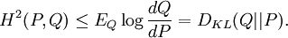
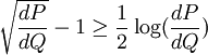
Noting that
Taking expectations with respect to Q, we get Other probability-distance measuresOther measures of probability distance are the histogram intersection, Chi-square statistic, quadratic form distance, match distance, Kolmogorov-Smirnov distance, and earth mover's distance (Rubner et al. 2000). See also
References
|
| This article is licensed under the GNU Free Documentation License. It uses material from the Wikipedia article "Kullback–Leibler_divergence". A list of authors is available in Wikipedia. |
 is to be finite) then
 , is the Radon-Nikodym derivative of P
with respect to Q and the expression becomes
, is the Radon-Nikodym derivative of P
with respect to Q and the expression becomes
 ,
,


 may be < = or > than
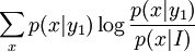
 may be < = or > than
 DKL( p(x|H1) || p(x|H0) ) .


 .
.
 or
or  , we see that
 .
.