To use all functions of this page, please activate cookies in your browser.
My watch list
my.chemeurope.com
my.chemeurope.com
With an accout for my.chemeurope.com you can always see everything at a glance – and you can configure your own website and individual newsletter.
- My watch list
- My saved searches
- My saved topics
- My newsletter
Differential entropy
Differential entropy (also referred to as continuous entropy) is a concept in information theory which tries to extend the idea of (Shannon) entropy, a measure of average surprisal of a random variable, to continuous probability distributions. Product highlight
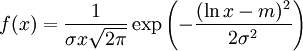
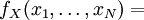
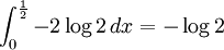
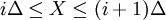
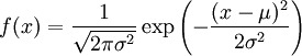
DefinitionLet X be a random variable with a probability density function f whose support is a set As with its discrete analog, the units of differential entropy depend on the base of the logarithm, which is usually 2 (i.e., the units are bits). See logarithmic units for logarithms taken in different bases. Related concepts such as joint, conditional differential entropy, and relative entropy are defined in a similar fashion. One must take care in trying to apply properties of discrete entropy to differential entropy, since probability density functions can be greater than 1. For example, Uniform(0,1/2) has differential entropy The definition of differential entropy above can be obtained by partitioning the range of X into bins of length Δ with associated sample points iΔ within the bins, for X Riemann integrable. This gives a quantized version of X, defined by XΔ = iΔ if
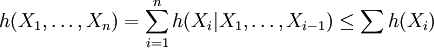
The first term approximates the differential entropy, while the second term is approximately − log(Δ). Note that this procedure suggests that the differential entropy of a discrete random variable should be Note that the continuous mutual information I(X;Y) has the distinction of retaining its fundamental significance as a measure of discrete information since it is actually the limit of the discrete mutual information of partitions of X and Y as these partitions become finer and finer. Thus it is invariant under quite general transformations of X and Y, and still represents the amount of discrete information that can be transmitted over a channel that admits a continuous space of values. Properties of differential entropy
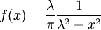
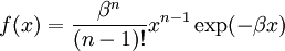
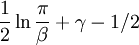
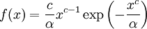
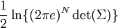
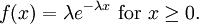
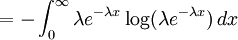
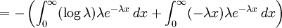
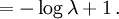
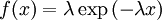
Example: Exponential distributionLet X be an exponentially distributed random variable with parameter λ, that is, with probability density function Its differential entropy is then
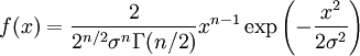
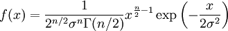
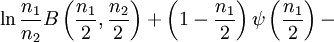
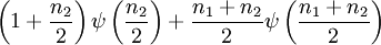
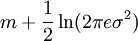
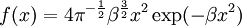
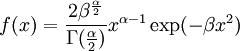
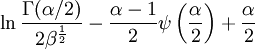
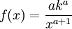
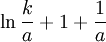
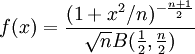
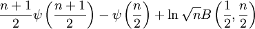
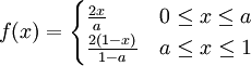
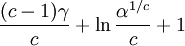
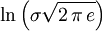
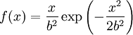
Here, he(X) was used rather than h(X) to make it explicit that the logarithm was taken to base e, to simplify the calculation. Differential entropies for various distributionsIn the table below,
See also
References
|
|||||||||||||||||||||||||||||||||||||||||||||||||||||||||||||||||||||||||||||
| This article is licensed under the GNU Free Documentation License. It uses material from the Wikipedia article "Differential_entropy". A list of authors is available in Wikipedia. |


 . The differential entropy
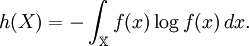
 .
.
 . Then the entropy of
 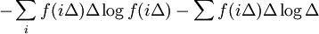 .
.
 .
.
 with equality if
 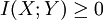 and
and  with equality if and only if X and Y are independent.
 .
.
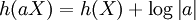 . For a vector valued random variable X and a matrix A,
  .
.
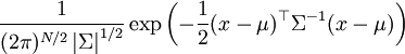
 has mean zero and covariance matrix K,
 ![h(\mathbf{X}) \leq \frac{1}{2} \log[(2\pi e)^n \det{K}]](images/math/5/0/3/503ffc96241b2575bfd151ab39010225.png) with equality if and only if X is jointly gaussian.
with equality if and only if X is jointly gaussian.

![= -\log \lambda \int_0^\infty f(x)\,dx + \lambda E[X]](images/math/1/1/1/111f140bd026b08482d9840334508dfd.png)
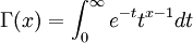 (the gamma function),
 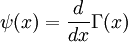 ,
, 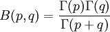 , and
, and 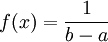 for
for 


 for
for 
![\ln B(p,q) - (p-1)[\psi(p) - \psi(p + q)] - (q-1)[\psi(q) - \psi(p + q)] \,](images/math/a/b/5/ab553119cbe12c724fa1955f79fbbc44.png)