To use all functions of this page, please activate cookies in your browser.
My watch list
my.chemeurope.com
my.chemeurope.com
With an accout for my.chemeurope.com you can always see everything at a glance – and you can configure your own website and individual newsletter.
- My watch list
- My saved searches
- My saved topics
- My newsletter
Linear elasticity
Linear elasticity is the mathematical study of how solid objects deform and become internally stressed due to prescribed loading conditions. Linear elasticity relies upon the continuum hypothesis and is applicable at macroscopic (and sometimes microscopic) length scales. Linear elasticity is a simplification of the more general nonlinear theory of elasticity and is a branch of continuum mechanics. The fundamental "linearizing" assumptions of linear elasticity are: "small" deformations (or strains) and linear relationships between the components of stress and strain. In addition linear elasticity is only valid for stress states that do not produce yielding. These assumptions are reasonable for many engineering materials and engineering design scenarios. Linear elasticity is therefore used extensively in structural analysis and engineering design, often through the aid of finite element analysis. This article presents a summary of some of the basic equations used to describe linear elasticity mathematically in tensor notation. For an alternative presentation using engineering notation, see the article on 3-D elasticity. Product highlight
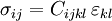
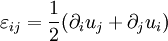
Basic equationsLinear elastodynamics is based on three tensor equations:
where:
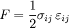
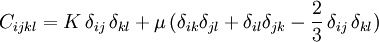
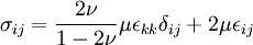
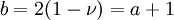
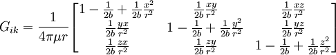
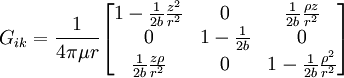
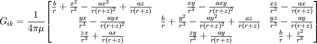
The basic elastostatic equations are given by setting Just as a spring which is compressed or expanded holds potential energy, so a strained material will possess an energy density due to the deformation. The energy density due to deformation is given by: Isotropic homogeneous mediaIn isotropic media, the elasticity tensor has the form where K is the bulk modulus (or incompressibility), and μ is the shear modulus (or rigidity), two elastic moduli. If the material is homogeneous (i.e. the elasticity tensor is constant throughout the material), the three basic equations can be combined to form the elastodynamic equation: and the constitutive equation may be written: Elastostatics - the elastostatic equationIf we assume that a steady state has been achieved, in which there is no time dependence to any of the quantities involved, the elastodynamic equation becomes the elastostatic equation Thomson's solution: point force at the origin of an infinite mediumThe most important solution of this equation is for that of a force acting at a point in an infinite isotropic medium. This solution was found by William Thomson (later Lord Kelvin) in 1848 (Thomson 1848). This solution is the analog of Coulomb's law in electrostatics. A derivation is given in (Landau & Lifshitz § 8). Defining where / nu is Poisson's ratio, the solution may be expressed as ui = Gikfk where fk is the force vector being applied at the point, and Gik is a tensor Green's function which may be written in Cartesian coordinates as: It may be also compactly written as: and it may be explicitly written as: In cylindrical coordinates (ρ,φ,z) it may be written as: It is particularly helpful to write the displacement in cylindrical coordinates for a point force Fz directed along the z-axis. Defining It can be seen that there is a component of the displacement in the direction of the force, which diminishes, as is the case for the potential in electrostatics, as 1/r. There is also an additional ρ-directed component. Boussinesq's solution - point force at the origin of an infinite isotropic half-spaceAnother useful solution is that of a point force acting on the surface of an infinite half-space. It was derived by Boussinesq(Boussinesq 1885) and a derivation is given in (See Landau & Lifshitz § 8). In this case, the solution is again written as a Green's tensor which goes to zero at infinity, and the component of the stress tensor normal to the surface vanishes. This solution may be written as in Cartesian coordinates as: Other solutions:
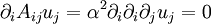
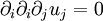
The biharmonic equationThe elastostatic equation may be written: Taking the divergence of both sides of the elastostatic equation and assuming a conservative force, ( Noting that summed indices need not match, and that the partial derivatives commute, the two differential terms are seen to be the same and we have: from which we conclude that: Taking the Laplacian of both sides of the elastostatic equation, a conservative force will give From the divergence equation, the first term on the right is zero (Note: again, the summed indices need not match) and we have: from which we conclude that: or, in coordinate free notation Elastodynamics - The Wave equationFrom the elastodynamic equation one gets the wave equation where is the acoustic differential operator, and δkl is Kronecker delta. In isotropic media, the elasticity tensor has the form where K is the bulk modulus (or incompressibility), and μ is the shear modulus (or rigidity), two elastic moduli. If the material is homogeneous (i.e. the elasticity tensor is constant throughout the material), the acoustic operator becomes: and the acoustic algebraic operator becomes where are the eigenvalues of Plane wavesA plane wave has the form with This propagation condition may be written as where
See also
References
|
|||
| This article is licensed under the GNU Free Documentation License. It uses material from the Wikipedia article "Linear_elasticity". A list of authors is available in Wikipedia. |


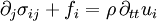
 is the Cauchy
  is the body force
 is the mass density
 is the displacement
 is the
  is the strain
 is the partial derivative
  and
and  is
is  .
.


![G_{ik}= \frac{1}{4\pi\mu r}\left[ \left(1-\frac{1}{2b}\right)\delta_{ik}+\frac{1}{2b}\frac{x_i x_k}{r^3} \right]](images/math/2/5/e/25e615cd64ef44b739bb74f6e46890c8.png)
![G_{ik}= \frac{1}{4\pi\mu}\left[\frac{\delta_{ik}}{r}-\frac{1}{2b}\frac{\partial r^2}{\partial x_i\partial x_k}\right]](images/math/0/8/e/08eb8b175cad8fabfb54aa45f353ebb3.png)
 and
and  as unit vectors in the
 ![\mathbf{u}=\frac{f_z}{4\pi\mu r}\left[\frac{1}{4(1-\nu)}\,\frac{\rho z}{r^2}\hat{\mathbf{\rho}} + \left(1-\frac{1}{4(1-\nu)}\,\frac{\rho^2}{r^2}\right)\hat{\mathbf{z}}\right]](images/math/c/c/e/cce4afd7a86cec0663138756a4346d8e.png)

 ) we have

 and we have


 which is just the biharmonic equation in
  .
.
![(\delta_{kl} \partial_{tt}-A_{kl}[\nabla]) \, u_l = \frac{1}{\rho} f_k](images/math/8/8/8/888bbbca42bfb2ccd912c19ee331cbca.png)
![A_{kl}[\nabla]=\frac{1}{\rho} \, \partial_i \, C_{iklj} \, \partial_j](images/math/2/8/9/289b0c6f9667496b2bcd9f876f5dc769.png)
![A_{ij}[\nabla]=\alpha^2 \partial_i\partial_j+\beta^2(\partial_m\partial_m\delta_{ij}-\partial_i\partial_j)\,](images/math/7/c/5/7c52f5a8a88f6fc0122015e07fdf2636.png)
![A_{ij}[\mathbf{k}]=\alpha^2 k_ik_j+\beta^2(k_mk_m\delta_{ij}-k_ik_j)\,](images/math/c/a/2/ca24bae0363bf3fc876cc64356ae9515.png)
![A[\hat{\mathbf{k}}]](images/math/e/e/9/ee92f1c15f30fa1d879640052bb973c1.png) with eigenvectors
with eigenvectors  parallel and orthogonal to the propagation direction
  , respectively. In the seismological literature, the corresponding plane waves are called P-waves and S-waves (see Seismic wave).
![\mathbf{u}[\mathbf{x}, \, t] = U[\mathbf{k} \cdot \mathbf{x} - \omega \, t] \, \hat{\mathbf{u}}](images/math/6/c/e/6cefbe907d062c9c559aa1b587bdbdb7.png)
![A_{kl}[\mathbf{k}]=\frac{1}{\rho} \, k_i \, C_{iklj} \, k_j](images/math/f/6/5/f651726c70b54b7e14117fda2d87f340.png)
![A[\hat{\mathbf{k}}] \, \hat{\mathbf{u}}=c^2 \, \hat{\mathbf{u}}](images/math/a/d/d/add5f05b98ab51bb899561f099639b41.png)
 denotes propagation direction
and
denotes propagation direction
and  is phase velocity.


