My watch list

3-D elasticity

It has been suggested that this article or section be merged into Linear elasticity. (Discuss)

3-D elasticity is one of three methods of structural analysis. This method is used for analyzing structures that behave in a linearly elastic fashion. There are 15 partial differential equations that must be simultaneously solved to get the state of stress at any point in an arbitrary structure. These are categorized into equilibrium, strain-displacement (or kinematic) relations, and the constitutive equations (or the general form of Hooke's law). Over the whole field the compatibility condition must be satisfied, which simply states that the displacement field is continuous and single-valued.

Additional recommended knowledge

How to ensure accurate weighing results every day?

Daily Visual Balance Check

Better weighing performance in 6 easy steps

1 Equilibrium equations
2 Strain-displacement equations
3 Constitutive equations
4 Compatibility equations
5 See also
6 References

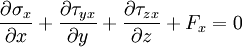
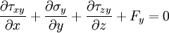
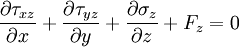
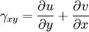
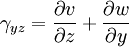
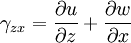
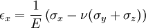
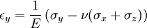
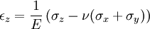
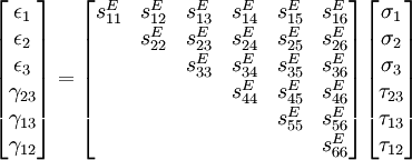
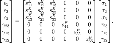
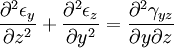
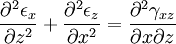
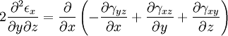
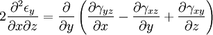
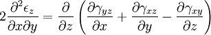
Equilibrium equations

The equilibrium equations of 3-D elasticity are formulated through the principle of conservation of linear momentum (i.e., Newton's second law of motion) as applied to a continuum. The equations may be expressed in Cartesian coordinates as

$\frac{\partial \sigma_x}{\partial x} + \frac{\partial \tau_{yx}}{\partial y} + \frac{\partial \tau_{zx}}{\partial z} + F_x = 0$

$\frac{\partial \tau_{xy}}{\partial x} + \frac{\partial \sigma_y}{\partial y} + \frac{\partial \tau_{zy}}{\partial z} + F_y = 0$

$\frac{\partial \tau_{xz}}{\partial x} + \frac{\partial \tau_{yz}}{\partial y} + \frac{\partial \sigma_z}{\partial z} + F_z = 0$

Where $σ i$ and $τ i j$ are the components of the Cauchy stress tensor which are defined as the current (or true) force per unit of deformed area; where $σ i$ is the normal stress in the i direction and $τ i j$ is the shear stress on the i face in the j direction.

$F i$ is called the body force and acts in the i direction. Body forces are generally known quantities. Common examples include gravity and electromagnetic forces. In structural analysis, body forces are sometimes small in comparison with applied loads and in such cases may be neglected.

The solution of the equilibrium equations fully defines the nine stress components throughout a structure. The conservation of angular momentum principle, however, reveals that not all nine of the stress components are independent. This principle shows that in the absence of body couples the stress tensor is symmetric (i.e., $τ i j = τ j i$ ) and the number of unknown stress components is reduced to six.

In general the equations of equilibrium cannot be solved without introducing additional equations. In other words, 3-D elastic structures are statically indeterminate.

Strain-displacement equations

The 3-D strain-displacement equations are as follows:

$\epsilon_x=\frac{\partial u}{\partial x}$

$\epsilon_y=\frac{\partial v}{\partial y}$

$\epsilon_z=\frac{\partial w}{\partial z}$

$\gamma_{xy}=\frac{\partial u}{\partial y} + \frac{\partial v}{\partial x}$

$\gamma_{yz}=\frac{\partial v}{\partial z} + \frac{\partial w}{\partial y}$

$\gamma_{zx}=\frac{\partial u}{\partial z} + \frac{\partial w}{\partial x}$

where $ε i$ is the normal strain in the i direction, $γ i j$ is the shear strain in the ij plane, and u, v, and w are the respective displacements in the x, y, and z directions.

These equations have 9 more unknown quantities, and only six more equations. With equilibrium there are a total of 15 unknowns and 9 equations. They cannot be solved yet.

Constitutive equations

The constitutive equation (or generalized 3-D Hooke's law) is as follows:

$\epsilon_x = \frac{1}{E}\left( \sigma_x - \nu(\sigma_y+\sigma_z) \right)$

$\epsilon_y = \frac{1}{E}\left( \sigma_y - \nu(\sigma_x+\sigma_z) \right)$

$\epsilon_z = \frac{1}{E}\left( \sigma_z - \nu(\sigma_x+\sigma_y) \right)$

$\gamma_{xy} = \frac{\tau_{xy}}{G}$

$\gamma_{yz} = \frac{\tau_{yz}}{G}$

$\gamma_{xz} = \frac{\tau_{xz}}{G}$

where E is the modulus of elasticity, ν is Poisson's ratio, G is the shear modulus, and all other variables are as defined above.

Since no new unknowns were introduced while 6 more independent equations now exist, it is possible to solve for the state of stress at an arbitrary point. Once this is done for every point in a body, compatibility must be satisfied for the displacement field to be physically possible.

For non-isotropic materials, this may be written in matrix form as

$\begin{bmatrix} \epsilon_1 \\ \epsilon_2 \\ \epsilon_3 \\ \gamma_{23} \\ \gamma_{13} \\ \gamma_{12} \end{bmatrix} = \begin{bmatrix} s_{11}^E & s_{12}^E & s_{13}^E & s_{14}^E & s_{15}^E & s_{16}^E \\ & s_{22}^E & s_{23}^E & s_{24}^E & s_{25}^E & s_{26}^E \\ & & s_{33}^E & s_{34}^E & s_{35}^E & s_{36}^E \\ & & & s_{44}^E & s_{45}^E & s_{46}^E \\ & & & & s_{55}^E & s_{56}^E \\ & & & & & s_{66}^E \end{bmatrix} \begin{bmatrix} \sigma_1 \\ \sigma_2 \\ \sigma_3 \\ \tau_{23} \\ \tau_{13} \\ \tau_{12} \end{bmatrix}$

with s₁₁^E = 1/Y₁₁, s₂₂^E = 1/Y₂₂, s₃₃^E = 1/Y₃₃, s₁₂^E = minus;ν₁₂/Y₁₁, etc.

where s_ij, the symmetric compliance matrix, with 21 independent constants.

In isotropic and orthotropic materials symmetry reduces the equations to:

$\begin{bmatrix} \epsilon_1 \\ \epsilon_2 \\ \epsilon_3 \\ \gamma_{23} \\ \gamma_{13} \\ \gamma_{12} \end{bmatrix} = \begin{bmatrix} s_{11}^E & s_{12}^E & s_{13}^E & 0 & 0 & 0 \\ s_{12}^E & s_{22}^E & s_{23}^E & 0 & 0 & 0 \\ s_{13}^E & s_{23}^E & s_{33}^E & 0 & 0 & 0 \\ 0 & 0 & 0 & s_{44}^E & 0 & 0 \\ 0 & 0 & 0 & 0 & s_{55}^E & 0 \\ 0 & 0 & 0 & 0 & 0 & s_{66}^E \end{bmatrix} \begin{bmatrix} \sigma_1 \\ \sigma_2 \\ \sigma_3 \\ \tau_{23} \\ \tau_{13} \\ \tau_{12} \end{bmatrix}.$

Compatibility equations

The 3-D equations of compatibility may be derived directly from the strain-displacement equations. They are as follows:

$\frac{\partial^2 \epsilon_x}{\partial y^2} + \frac{\partial^2 \epsilon_y}{\partial x^2} = \frac{\partial^2 \gamma_{xy}}{\partial x \partial y}$

$\frac{\partial^2 \epsilon_y}{\partial z^2} + \frac{\partial^2 \epsilon_z}{\partial y^2} = \frac{\partial^2 \gamma_{yz}}{\partial y \partial z}$

$\frac{\partial^2 \epsilon_x}{\partial z^2} + \frac{\partial^2 \epsilon_z}{\partial x^2} = \frac{\partial^2 \gamma_{xz}}{\partial x \partial z}$

$2 \frac{\partial^2 \epsilon_x}{\partial y \partial z} = \frac{\partial}{\partial x} \left ( -\frac{\partial \gamma_{yz}}{\partial x} + \frac{\partial \gamma_{xz}}{\partial y} + \frac{\partial \gamma_{xy}}{\partial z}\right)$

$2 \frac{\partial^2 \epsilon_y}{\partial x \partial z} = \frac{\partial}{\partial y} \left ( \frac{\partial \gamma_{yz}}{\partial x} - \frac{\partial \gamma_{xz}}{\partial y} + \frac{\partial \gamma_{xy}}{\partial z}\right)$

$2 \frac{\partial^2 \epsilon_z}{\partial x \partial y} = \frac{\partial}{\partial z} \left ( \frac{\partial \gamma_{yz}}{\partial x} + \frac{\partial \gamma_{xz}}{\partial y} - \frac{\partial \gamma_{xy}}{\partial z}\right)$

References

A.C. Ugural, S.K. Fenster, Advanced Strength and Applied Elasticity, 4th ed.

Categories: Continuum mechanics | Materials science

This article is licensed under the GNU Free Documentation License. It uses material from the Wikipedia article "3-D_elasticity". A list of authors is available in Wikipedia.

3-D elasticity

Additional recommended knowledge

How to ensure accurate weighing results every day?

Daily Visual Balance Check

Better weighing performance in 6 easy steps

Contents

Equilibrium equations

Strain-displacement equations

Constitutive equations

Compatibility equations

See also

References

About chemeurope.com

About LUMITOS

Advertise with LUMITOS