My watch list

Home
Encyclopedia
Sinusoidal_plane-wave_solutions_of_the_electromagnetic_wave_equation

Sinusoidal plane-wave solutions of the electromagnetic wave equation

Perhaps the most useful solutions to the electromagnetic wave equation are sinusoidal plane-wave solutions. The general solution of the electromagnetic wave equation can be written as a linear superposition of plane-waves of different frequencies and polarizations. Experimentally, every light signal can be decomposed into a spectrum of frequencies and wavelengths associated with sinusoidal solutions of the wave equation. Polarizing filters can be used to decompose light into its various polarization components. The polarization components can be linear, circular or elliptical.

The treatment in this article is classical. It is a testament, however, to the generality of Maxwell's equations for electrodynamics that the treatment can be made to be quantum mechanical with only a reinterpretation of classical quantities. The reinterpretation is based on the experiments of Max Planck and the interpretations of those experiments by Albert Einstein. The quantum generalization of the classical treatment can be found in the articles on Photon polarization and Photon dynamics in the double-slit experiment.

Additional recommended knowledge

Daily Sensitivity Test

Guide to balance cleaning: 8 simple steps

What is the Correct Way to Check Repeatability in Balances?

1 Plane waves
2 Polarization state vector
3 Polarization states
4 References
5 See also

Plane waves

The plane sinusoidal solution for an electromagnetic wave traveling in the z direction is (cgs units and SI units)

$\mathbf{E} ( \mathbf{r} , t ) = \begin{pmatrix} E_x^0 \cos \left ( kz-\omega t + \alpha_x \right ) \\ E_y^0 \cos \left ( kz-\omega t + \alpha_y \right ) \\ 0 \end{pmatrix} = E_x^0 \cos \left ( kz-\omega t + \alpha_x \right ) \hat {\mathbf{x}} \; + \; E_y^0 \cos \left ( kz-\omega t + \alpha_y \right ) \hat {\mathbf{y}}$

for the electric field and

$\mathbf{B} ( \mathbf{r} , t ) = \hat { \mathbf{z} } \times \mathbf{E} ( \mathbf{r} , t ) = \begin{pmatrix} -E_y^0 \cos \left ( kz-\omega t + \alpha_y \right ) \\ E_x^0 \cos \left ( kz-\omega t + \alpha_x \right ) \\ 0 \end{pmatrix} = -E_y^0 \cos \left ( kz-\omega t + \alpha_y \right ) \hat {\mathbf{x}} \; + \; E_x^0 \cos \left ( kz-\omega t + \alpha_x \right ) \hat {\mathbf{y}}$

for the magnetic field, where k is the wavenumber,

$\omega_{ }^{ } = c k$

is the angular frequency of the wave, and $c$ is the speed of light. The hats on the vectors indicate unit vectors in the x, y, and z directions.

The plane wave is parameterized by the amplitudes

$E_x^0 = \mid \mathbf{E} \mid \cos \theta$

$E_y^0 = \mid \mathbf{E} \mid \sin \theta$

and phases

$\alpha_x^{ } , \alpha_y$

where

$\theta \ \stackrel{\mathrm{def}}{=}\ \tan^{-1} \left ( { E_y^0 \over E_x^0 } \right )$ .

and

$\mid \mathbf{E} \mid^2 \ \stackrel{\mathrm{def}}{=}\ \left ( E_x^0 \right )^2 + \left ( E_y^0 \right )^2$ .

Polarization state vector

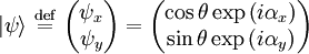
Jones vector

All the polarization information can be reduced to a single vector, called the Jones vector, in the x-y plane. This vector, while arising from a purely classical treatment of polarization, can be interpreted as a quantum state vector. The connection with quantum mechanics is made in the article on photon polarization.

The vector emerges from the plane-wave solution. The electric field solution can be re-written in complex notation as

$\mathbf{E} ( \mathbf{r} , t ) = \mid \mathbf{E} \mid \mathrm{Re} \left \{ |\psi\rangle \exp \left [ i \left ( kz-\omega t \right ) \right ] \right \}$

where

$|\psi\rangle \ \stackrel{\mathrm{def}}{=}\ \begin{pmatrix} \psi_x \\ \psi_y \end{pmatrix} = \begin{pmatrix} \cos\theta \exp \left ( i \alpha_x \right ) \\ \sin\theta \exp \left ( i \alpha_y \right ) \end{pmatrix}$

is the Jones vector in the x-y plane. The notation for this vector is the bra-ket notation of Dirac, which is normally used in a quantum context. The quantum notation is used here in anticipation of the interpretation of the Jones vector as a quantum state vector.

Dual Jones vector

The Jones vector has a dual given by

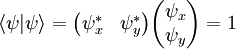
$\langle \psi | \ \stackrel{\mathrm{def}}{=}\ \begin{pmatrix} \psi_x^* & \psi_y^* \end{pmatrix} = \begin{pmatrix} \quad \cos\theta \exp \left ( -i \alpha_x \right ) & \sin\theta \exp \left ( -i \alpha_y \right ) \quad \end{pmatrix}$ .

Normalization of the Jones vector

The Jones vector is normalized. The inner product of the vector with itself is

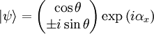
$\langle \psi | \psi\rangle = \begin{pmatrix} \psi_x^* & \psi_y^* \end{pmatrix} \begin{pmatrix} \psi_x \\ \psi_y \end{pmatrix} = 1$ .

Polarization states

Linear polarization

Main article: Linear polarization

In general, the wave is linearly polarized when the phase angles $\alpha_x^{ } , \alpha_y$ are equal,

$\alpha_x = \alpha_y \ \stackrel{\mathrm{def}}{=}\ \alpha$ .

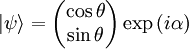
This represents a wave polarized at an angle $θ$ with respect to the x axis. In that case the Jones vector can be written

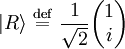
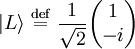
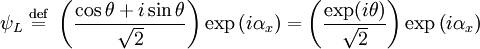
$|\psi\rangle = \begin{pmatrix} \cos\theta \\ \sin\theta \end{pmatrix} \exp \left ( i \alpha \right )$ .

Circular polarization

Main article: Circular polarization

If $α y$ is rotated by $π / 2$ radians with respect to $α x$ the wave is circularly polarized. The Jones vector is

$|\psi\rangle = \begin{pmatrix} \cos\theta \\ \pm i\sin\theta \end{pmatrix} \exp \left ( i \alpha_x \right )$

where the plus sign indicates right circular polarization and the minus sign indicates left circular polarization. In the case of circular polarization, the electric field vector of constant magnitude rotates in the x-y plane.

If unit vectors are defined such that

$|R\rangle \ \stackrel{\mathrm{def}}{=}\ {1 \over \sqrt{2}} \begin{pmatrix} 1 \\ i \end{pmatrix}$

and

$|L\rangle \ \stackrel{\mathrm{def}}{=}\ {1 \over \sqrt{2}} \begin{pmatrix} 1 \\ -i \end{pmatrix}$

then a circular polarization state can written in the "R-L basis" as

$|c\rangle = \psi_R |R\rangle + \psi_L |L\rangle$

where

$\psi_R \ \stackrel{\mathrm{def}}{=}\ \left ( {\cos\theta -i\sin\theta \over \sqrt{2} } \right ) \exp \left ( i \alpha_x \right ) = \left ( {\exp(-i\theta) \over \sqrt{2} } \right ) \exp \left ( i \alpha_x \right )$

and

$\psi_L \ \stackrel{\mathrm{def}}{=}\ \left ( {\cos\theta +i\sin\theta \over \sqrt{2} } \right ) \exp \left ( i \alpha_x \right ) = \left ( {\exp(i\theta) \over \sqrt{2} } \right ) \exp \left ( i \alpha_x \right )$ .

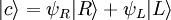
Any arbitrary state can be written in the R-L basis

$|\psi\rangle = a_R \exp \left ( i \alpha_x -i \theta \right ) |R\rangle + a_L \exp \left ( i \alpha_x + i \theta \right ) |L\rangle$

where

$1 = \mid a_R \mid^2 + \mid a_L \mid^2$ .

Elliptical polarization

Main article: Elliptical polarization

The general case in which the electric field rotates in the x-y plane and has variable magnitude is called elliptical polarization. The state vector is given by

References

Jackson, John D. (1998). Classical Electrodynamics (3rd ed.). Wiley. ISBN 0-471-30932-X.

Sinusoidal plane-wave solutions of the electromagnetic wave equation

Additional recommended knowledge

Daily Sensitivity Test

Guide to balance cleaning: 8 simple steps

What is the Correct Way to Check Repeatability in Balances?

Contents

Plane waves

Polarization state vector

Jones vector

Dual Jones vector

Normalization of the Jones vector

Polarization states

Linear polarization

Circular polarization

Elliptical polarization

References

See also

About chemeurope.com

About LUMITOS

Advertise with LUMITOS