To use all functions of this page, please activate cookies in your browser.
My watch list
my.chemeurope.com
my.chemeurope.com
With an accout for my.chemeurope.com you can always see everything at a glance – and you can configure your own website and individual newsletter.
- My watch list
- My saved searches
- My saved topics
- My newsletter
Surface plasmonSurface plasmons, also referred to in the literature as surface plasma polaritons, are fluctuations in the electron density at the boundary of two materials. Plasmons are the collective vibrations of an electron gas (or plasma) surrounding the atomic lattice sites of a metal. When plasmons couple with a photon, the resulting particle is called a polariton. This polariton propagates along the surface of the metal until it decays, either by absorption, whereupon the energy is converted into phonons, or by a radiative transition into a photon. Surface Plasmons were first reported in 1957 by R.H. Ritchie[1]. In the following two decades, Surface Plasmons were extensively studied by many scientists, the foremost of whom were Prof. Dr. Heinz Raether, E. Kretschmann, and A. Otto. Product highlight
ExcitationFigure 1: (a) Kretschmann and (b) Otto configuration of an Attenuated Total Reflection setup for coupling surface plasmons. In both cases, the surface plasmon propagates along the metal/dielectric interface Figure 2: Grating Coupler for Surface Plasmons. The wave vector is increased by the spatial frequency
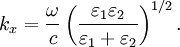
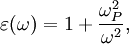
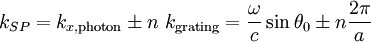
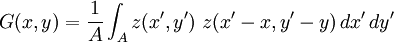
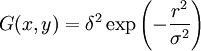
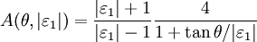
Surface plasmons can be excited by both electrons and photons. Excitation by electrons is realized by shooting electrons into a metal. As the electrons scatter, energy is transferred into the plasma. The component of the scattering vector parallel to the surface results in the formation of a surface plasmon. Excitation by photons requires the use of a coupling medium such as a prism or grating to match the photon and surface plasmon wave vectors. A prism can be positioned against a thin metal film in the Kretschmann configuration or very close to a metal surface in the Otto configuration (Figure 1). A grating coupler matches the wave vectors by increasing the wave vector by the spatial frequency of the grating (Figure 2). This method, while less frequently utilized, is critical to the theoretical understanding of the impact of surface roughness. Dispersion relationshipThe electric field of a propagating electromagnetic wave can be expressed where k is the wave number and ω is the frequency of the wave. By solving Maxwell's equations for the electromagnetic wave at an interface between two materials with relative dielectric constants and where c is the speed of light in a vacuum. Solving these two equations, the dispersion relationship for a wave propagating on the surface is In the free electron model of an electron gas, the dielectric constant is[3] where the plasma frequency is where n is the electron density, e is the charge of the electron, and m* is the effective mass of the electron. The dispersion relationship is plotted in Figure 4. At low k, the surface plasmon behaves like a photon, but as k increases, the dispersion relationship bends over and reaches an asymptotic limit. Since the dispersion curve lies to the right of the light curve, ω = k * c, the surface plasmon is non-radiative. Finally solving these equations, the maximum frequency of the surface plasmon is calculated to be In the case of air, this result simplifies to If we assume that The wave vector gives us insight into physically meaningful properties of the electromagnetic wave such as its spatial extent and coupling requirements for wave vector matching. Propagation length and skin depthAs a surface plasmon propagates along the surface, it quickly loses its energy to the metal due to absorption. The intensity of the surface plasmon decays with the square of the electric field, so at a distance x, the intensity has decreased by a factor of exp[ − 2kx''x]. The propagation length is defined as the distance for the surface plasmon to decay by a factor of 1 / e. This condition is satisfied at a length[4] Likewise, the electric field falls off exponentially normal to the surface. The skin depth is defined as the distance where the electric field falls off by 1 / e. The field will fall of at different rates in the metal and dielectric medium and the skin depth in each medium can be expressed[4] where i indicates the medium of propagation. Surface plasmons are very sensitive to slight perturbations within the skin depth and because of this, surface plasmons are often used to probe inhomogeneities of a surface. Effects of roughnessIn order to understand the effect of roughness on surface plasmons, it is beneficial to first understand how a plasmon is coupled by a grating (Figure 2). When a photon is incident on a surface, the wave vector of the photon in the dielectric material is smaller than that of the surface plasmon. In order for the photon to couple into a surface plasmon, the wave vector must increase by Δk = kSP − kx,photon. The harmonics of a periodic grating add to the wave vector to match the terms. where kgrating is the wave vector of the grating, θ0 is the angle of incidence of the incoming photon, a is the grating period, and n is an integer. Rough surfaces can be thought of as the superposition of many gratings of different periodicities. Kretschmann proposed[5] that a statistical correlation function be defined for a rough surface where z(x,y) is the height above the mean surface height at the position (x,y), and A is the area of integration. Assuming that the statistical correlation function is be Gaussian of the form where δ is the root mean square height, r is the distance from the point (x,y), and σ is the correlation length, then the Fourier transform of the correlation function is where s is a measure of the amount of each spatial frequency ksurf which help couple photons into a surface plasmon. If the surface only has one Fourier component of roughness (i.e. the surface profile is sinusoidal), then the s is discrete and exists only at As stated earlier, surface plasmons are non-radiative. When a surface plasmon travels along a rough surface, it usually becomes radiative due to scattering. The Surface Scattering Theory of light suggests that the scattered intensity dI per solid angle dΩ per incident intensity I0 is[6] where | W | 2 is the radiation pattern from a single dipole at the metal/dielectric interface. If surface plasmons are excited in the Kretschmann geometry and the scattered light is observed in the plane of incidence (Fig. 4), then the dipole function becomes with where ψ is the polarization angle and θ is the angle from the z-axis in the xz-plane. Two important consequences come out of these equations. The first is that if ψ = 0 (s-polarization), then | W | 2 = 0 and the scattered light Experimental applicationsThe excitation of surface plasmons is frequently used in an experimental technique known as surface plasmon resonance (SPR). In SPR, the maximum excitation of surface plasmons are detected by monitoring the reflected power from a prism coupler as a function of incident angle or wavelength. This technique can be used to observe nanometer changes in thickness, density fluctuations, or molecular adsorption. In surface second harmonic generation, the second harmonic signal is proportional to the square of the electric field. The electric field is stronger at the interface because of the surface plasmon. This larger signal is often exploited to produce a stronger second harmonic signal. References
Categories: Plasma physics | Condensed matter physics |
|
| This article is licensed under the GNU Free Documentation License. It uses material from the Wikipedia article "Surface_plasmon". A list of authors is available in Wikipedia. |


![E= E_{0}\exp[i(k_{x} x + k_{z} z -\omega t)]\,](images/math/0/6/a/06a818c3ccf10d99041557de0ba580f2.png)
 and
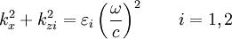
and  (see figure 3) with the appropriate continuity relationships the boundary conditions are found to be
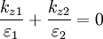
 , then it must be true that
  , a condition which is satisfied in metals. EM waves passing through a metal experience damping due to electrical conductivity and electron-core interactions. These effects show up in as an imaginary component of the
  where
where  and
and  are the real and imaginary parts of the dielectric function, respectively. Generally
  so the wavenumber can be expressed in terms of its real and imaginary components
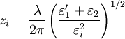
![k_{x}=k_{x}'+i k_{x}''=\left[\frac{\omega}{c} \left( \frac{\varepsilon_1' \varepsilon_2}{\varepsilon_1' + \varepsilon_2}\right)^{1/2}\right] + i \left[\frac{\omega}{c} \left( \frac{\varepsilon_1' \varepsilon_2}{\varepsilon_1' + \varepsilon_2}\right)^{3/2} \frac{\varepsilon_1''}{2(\varepsilon_1')^2}\right].](images/math/8/0/6/806548d4a83b85b84be5d3aca3dc678f.png)

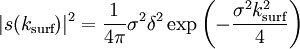
 , resulting in a single narrow set of angles for coupling. If the surface contains many Fourier components, then coupling becomes possible at multiple angles. For a random surface,
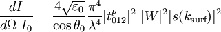
![|W|^2=A(\theta,|\varepsilon_{1}|)\ \sin^2{\psi} \ [(1+\sin^2 \theta /|\varepsilon_1|)^{1/2} - \sin{\theta}]^2](images/math/b/7/2/b727f993c57727e22a639c73127fec30.png)
 . Secondly, the scattered light has a measurable profile which is readily correlated to the roughness. This topic is treated in greater detail in reference
 Last viewed


