To use all functions of this page, please activate cookies in your browser.
My watch list
my.chemeurope.com
my.chemeurope.com
With an accout for my.chemeurope.com you can always see everything at a glance – and you can configure your own website and individual newsletter.
- My watch list
- My saved searches
- My saved topics
- My newsletter
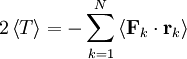
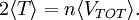
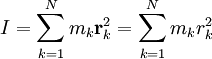
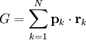
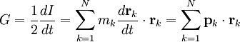
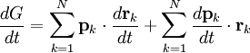
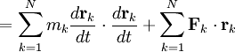
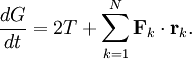
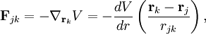
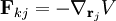
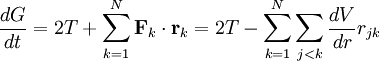
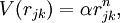
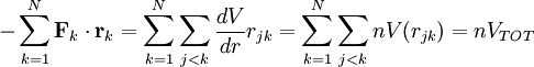
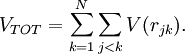
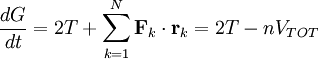
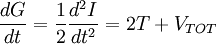
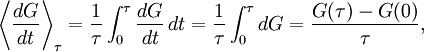
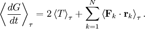
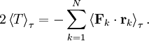
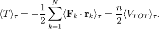
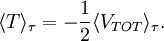
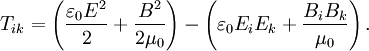
Virial theoremIn mechanics, the virial theorem provides a general equation relating the average total kinetic energy where Fk represents the force on the kth particle, which is located at position rk. The word "virial" derives from vis, the Latin word for "force" or "energy", and was given its technical definition by Clausius in 1870.[1] Fritz Zwicky was the first to use the virial theorem to deduce the existence of unseen matter, what is now called dark matter. The significance of the virial theorem is that it allows the average total kinetic energy to be calculated even for very complicated systems that defy an exact solution, such as those considered in statistical mechanics; this average total kinetic energy is related to the temperature of the system by the equipartition theorem. However, the virial theorem does not depend on the notion of temperature and holds even for systems that are not in thermal equilibrium. The virial theorem has been generalized in various ways, most notably to a tensor form. If the force between any two particles of the system results from a potential energy V(r)=αr n that is proportional to some power n of the inter-particle distance r, the virial theorem adopts a simple form Thus, twice the average total kinetic energy Although the virial theorem depends on averaging the total kinetic and potential energies, the presentation here postpones the averaging to the last step; please be patient! Product highlightDefinitions of the virial and its time derivativeFor a collection of N point particles, the scalar moment of inertia I about the origin is defined by the equation where mk and rk represent the mass and position of the kth particle. The scalar virial G is defined by the equation where pk is the momentum vector of the kth particle. Assuming that the masses are constant, the virial G is the time derivative of this moment of inertia In turn, the time derivative of the virial G can be written or, more simply, Here mk is the mass of the kth particle, Connection with the potential energy between particlesThe total force where Since no particle acts on itself (i.e., where we have assumed that Newton's third law of motion holds, i.e., It often happens that the forces can be derived from a potential energy V that is a function only of the distance rjk between the point particles j and k. Since the force is the gradient of the potential energy, we have in this case which is clearly equal and opposite to Thus, we have Special case of power-law forcesIn a common special case, the potential energy V between two particles is proportional to a power n of their distance r where the coefficient α and the exponent n are constants. In such cases, the force term of the virial time derivative is given by the equation where VTOT is the total potential energy of the system Thus, we have For gravitating systems and also for electrostatic systems, the exponent n equals -1, giving Lagrange's identity which was derived by Lagrange and extended by Jacobi. Time averaging and the virial theoremThe average of this derivative over a time τ is defined as from which we obtain the exact equation The virial theorem states that, if There are many reasons why the average of the time derivative might vanish, i.e., Even if the average of the time derivative For power-law forces with an exponent n, the general equation holds For gravitational attraction, n equals -1 and the average kinetic energy equals half of the average negative potential energy This general result is useful for complex gravitating systems such as solar systems or galaxies. A simple application of the Virial theorem concerns galaxy clusters. If a region of space is unusually full of galaxies, it is safe to assume that they have been together for a long time, and the Virial theorem can be applied. Doppler measurements give lower bounds for their relative velocities, and the Virial theorem gives a lower bound for the total mass of the cluster, including any dark matter. The averaging need not be taken over time; an ensemble average can also be taken, with equivalent results. Although derived for classical mechanics, the virial theorem also holds for quantum mechanics. Generalizations of the virial theoremLord Rayleigh published a generalization of the virial theorem in 1903.[2] Henri Poincaré applied a form of the virial theorem in 1911 to the problem of determining cosmological stability.[3] A variational form of the virial theorem was developed in 1945 by Ledoux.[4] A tensor form of the virial theorem was developed by Parker,[5] Chandrasekhar[6] and Fermi.[7] Inclusion of electromagnetic fieldsThe virial theorem can be extended to include electric and magnetic fields. The result is[8] where I is the moment of inertia, G is the momentum density of the electromagnetic field, T is the kinetic energy of the "fluid", U is the random "thermal" energy of the particles, WE and WM are the electric and magnetic energy content of the volume considered. Finally, pik is the fluid-pressure tensor expressed in the local moving coordinate system
and Tik is the electromagnetic stress tensor, A plasmoid is a finite configuration of magnetic fields and plasma. With the virial theorem it is easy to see that any such configuration will expand if not contained by external forces. In a finite configuration without pressure-bearing walls or magnetic coils, the surface integral will vanish. Since all the other terms on the right hand side are positive, the acceleration of the moment of inertia will also be positive. It is also easy to estimate the expansion time τ. If a total mass M is confined within a radius R, then the moment of inertia is roughly MR2, and the left hand side of the virial theorem is MR2/τ2. The terms on the right hand side add up to about pR3, where p is the larger of the plasma pressure or the magnetic pressure. Equating these two terms and solving for τ, we find where cs is the speed of the ion acoustic wave (or the Alfven wave, if the magnetic pressure is higher than the plasma pressure). Thus the lifetime of a plasmoid is expected to be on the order of the acoustic (or Alfven) transit time. Virial radiusIn astronomy, the term virial radius is sometimes used to refer to the radius of a sphere, centered on a galaxy or a galaxy cluster, within which the average density is greater, by a specified factor, than the critical density See also
References
Additional reading
External Links
|
| This article is licensed under the GNU Free Documentation License. It uses material from the Wikipedia article "Virial_theorem". A list of authors is available in Wikipedia. |
 of a system with its average total potential energy
  , where angle brackets represent the average of the enclosed quantity. Mathematically, the virial theorem states


 is the net force on that particle and
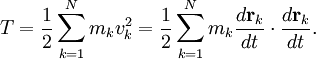
 on particle
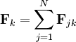
 is the force applied by particle
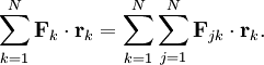
 whenever
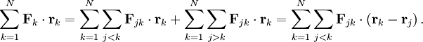
 (equal and opposite reaction).
 , the force applied by particle
 , then

 is only approximately zero, the virial theorem holds to the same degree of approximation.

 ,
,

 . (Here, H is the Hubble parameter and G is the gravitational constant.) A common choice for the factor is 200, in which case the virial radius is designated as

