To use all functions of this page, please activate cookies in your browser.
My watch list
my.chemeurope.com
my.chemeurope.com
With an accout for my.chemeurope.com you can always see everything at a glance – and you can configure your own website and individual newsletter.
- My watch list
- My saved searches
- My saved topics
- My newsletter
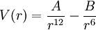
Lennard-Jones potentialNeutral atoms and molecules are subject to two distinct forces in the limit of large distance and short distance: an attractive force at long ranges (van der Waals force, or dispersion force) and a repulsive force at short ranges (the result of overlapping electron orbitals, referred to as Pauli repulsion from Pauli exclusion principle). The Lennard-Jones potential (also referred to as the L-J potential, 6-12 potential or, less commonly, 12-6 potential) is a simple mathematical model that represents this behavior. It was proposed in 1924 by John Lennard-Jones.[1] The L-J potential is of the form where These parameters can be fitted to reproduce experimental data or deduced from results of accurate quantum chemistry calculations. The
The lowest energy arrangement of an infinite number of atoms described by a Lennard-Jones potential is a hexagonal close-packing. On raising temperature, the lowest free energy arrangement becomes cubic close packing and then liquid. Under pressure the lowest energy structure switches between cubic and hexagonal close packing.[2] Other more recent methods, such as the Stockmayer equation and the so-called multi equation, describe the interaction of molecules more accurately. Quantum chemistry methods, Møller-Plesset perturbation theory, coupled cluster method or full configuration interaction can give extremely accurate results, but require large computational cost. Product highlight
Alternative expressionsThe Lennard-Jones potential function is also often written as where
The simplest formulation, often used internally by simulation software, is:
where
and
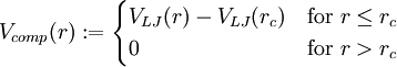
Molecular dynamics simulation: Truncated potentialTo save computational time, the Lennard-Jones (LJ) potential
is often truncated at the cut-off distance of
i.e., at
For clarity, let
The computational potential
It can be easily verified that
See also
References
Categories: Thermodynamics | Chemical bonding | Intermolecular forces | Computational chemistry |
|||||||
| This article is licensed under the GNU Free Documentation License. It uses material from the Wikipedia article "Lennard-Jones_potential". A list of authors is available in Wikipedia. |
![V(r) = 4\epsilon \left[ \left(\frac{\sigma}{r}\right)^{12} - \left(\frac{\sigma}{r}\right)^{6} \right]](images/math/e/a/c/eac9407d601624e0d5123ae78ccc1127.png)
 is the depth of the potential well and
  is the (finite) distance at which the interparticle potential is zero.
 term describes repulsion and the
 term describes attraction.
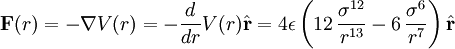
The force function is the negative of the gradient of the above potential:
term describes attraction.
The force function is the negative of the gradient of the above potential:


![V(r) = \epsilon \left[ \left(\frac{r_{min}}{r}\right)^{12} - 2\left(\frac{r_{min}}{r}\right)^{6} \right]](images/math/d/9/2/d9283be3ed70576130d56caa6710c081.png)
 =
=  is the distance at the minimum of the potential.


 .
.
 where
where
![\displaystyle V ( r_c ) = V ( 2.5 \sigma ) = 4 \epsilon \left[ \left( \frac {\sigma} {2.5 \sigma} \right)^{12} - \left( \frac {\sigma} {2.5 \sigma} \right)^6 \right] = -0.0163 \epsilon = - \frac {1} {61.3} \epsilon](images/math/b/e/f/bef09563e5795f7567db0ac31a3378f7.png)
 is about 1/60th of its minimum value
 (depth of potential well).
Beyond
(depth of potential well).
Beyond
 , the computational potential
is set to zero.
On the other hand, to avoid a jump discontinuity at
, the computational potential
is set to zero.
On the other hand, to avoid a jump discontinuity at
 denote the LJ potential as defined above, i.e.,
![\displaystyle V_{LJ} (r) = 4 \epsilon \left[ \left( \frac {\sigma} {r} \right)^{12} - \left( \frac {\sigma} {r} \right)^6 \right]](images/math/7/7/7/777dac5a547800612f7ea372599eaff5.png)
 is defined as follows
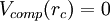 ,
thus eliminating the jump discontinuity at
,
thus eliminating the jump discontinuity at
 .
.


