To use all functions of this page, please activate cookies in your browser.
My watch list
my.chemeurope.com
my.chemeurope.com
With an accout for my.chemeurope.com you can always see everything at a glance – and you can configure your own website and individual newsletter.
- My watch list
- My saved searches
- My saved topics
- My newsletter
Potts modelIn statistical mechanics, the Potts model, a generalization of the Ising model, is a model of interacting spins on a crystalline lattice. By studying the Potts model, one may gain insight into the behaviour of ferromagnets and certain other phenomena of solid state physics. The strength of the Potts model is not so much that it models these physical systems well; it is rather that the one-dimensional case is exactly solvable, and that it has a rich mathematical formulation that has been studied extensively. The model is named after Renfrey B. Potts who described the model near the end of his 1952 Ph.D. thesis. The model was related to the "planar Potts" or "clock model", which was suggested to him by his advisor Cyril Domb. The Potts model is sometimes known as the Ashkin-Teller model (after Julius Ashkin and Edward Teller), as they considered a four component version in 1943. The Potts model is related to, and generalized by, several other models, including the XY model, the Heisenberg model and the N-vector model. The infinite-range Potts model is known as the Kac model. When the spins are taken to interact in a non-Abelian manner, the model is related to the flux tube model, which is used to discuss confinement in quantum chromodynamics. Generalizations of the Potts model have also been used to model grain growth in metals and coarsening in foams. A further generalization of these methods by James Glazier and Francois Graner, known as the Cellular Potts Model has been used to simulate static and kinetic phenomena in foam and biological morphogenesis. Product highlight
Physical descriptionThe Potts model consists of spins that are placed on a lattice; the lattice is usually taken to be a two-dimensional rectangular Euclidean lattice, but is often generalized to other dimensions or other lattices. Domb originally suggested that the spin take one of q possible values, distributed uniformly about the circle, at angles and that the interaction Hamiltonian be given by with the sum running over the nearest neighbor pairs (i,j) over all lattice sites. The site colors si take on values, ranging from What is now known as the standard Potts model was suggested by Potts in the course of the solution above, and uses a simpler Hamiltonian, given by: where δ(si,sj) is the Kronecker delta, which equals one whenever si = sj and zero otherwise. The q=2 standard Potts model is equivalent to the 2D Ising model and the 2-state vector Potts model, with Jp = − 2Jc. The q=3 standard Potts model is equivalent to the three-state vector Potts model, with Jp = − 3Jc / 2. A common generalization is to introduce an external "magnetic field" term h, and moving the parameters inside the sums and allowing them to vary across the model: where β = 1 / kT the inverse temperature, k the Boltzmann constant and T the temperature. The summation may run over more distant neighbors on the lattice, or may in fact be an infinite-range force. Different papers may adopt slightly different conventions, which can alter H and the associated partition function by additive or multiplicative constants. DiscussionDespite its simplicity as a model of a physical system, the Potts model is useful as a model system for the study of phase transitions. For example 2D dimensional lattices with J > 0 exhibit a first order transition if q > 4. When The model has a close relation to the Fortuin-Kasteleyn random cluster model, another model in statistical mechanics. Understanding this relationship has helped develop efficient Markov chain Monte Carlo methods for numerical exploration of the model at small q. Measure theoretic descriptionThe one dimensional Potts model may be expressed in terms of a subshift of finite type, and thus gains access to all of the mathematical techniques associated with this formalism. In particular, it can be solved exactly using the techniques of transfer operators. (However, Ernst Ising used combinatorial methods to solve the Ising model, which is the "ancestor" of the Potts model, in his 1925 PhD thesis). This section develops the mathematical formalism, based on measure theory, behind this solution. While the example below is developed for the one-dimensional case, many of the arguments, and almost all of the notation, generalizes easily to any number of dimensions. Some of the formalism is also broad enough to handle related models, such as the XY model, the Heisenberg model and the N-vector model. Topology of the space of statesLet be the set of all bi-infinite strings of values from the set Q. This set is called a full shift. For defining the Potts model, either this whole space, or a certain subset of it, a subshift of finite type, may be used. Shifts get this name because there exists a natural operator on this space, the shift operator
This set has a natural product topology; the base for this topology are the cylinder sets that is, the set of all possible strings where k+1 spins match up exactly to a given, specific set of values Interaction energyThe interaction between the spins is then given by a continuous function
will be seen to describe the interaction between nearest neighbors. Of course, different functions give different interactions; so a function of s0, s1 and s2 will describe a next-nearest neighbor interaction. A function V gives interaction energy between a set of spins; it is not the Hamiltonian, but is used to build it. The argument to the function V is an element Define the function This function can be seen to consist of two parts: the self-energy of a configuration Partition function and measureThe corresponding finite-state partition function is given by with C0 being the cylinder sets defined above. Here, β=1/kT, where k is Boltzmann's constant, and T is the temperature. It is very common in mathematical treatments to set β=1, as it is easily regained by rescaling the interaction energy. This partition function is written as a function of the interaction V to emphasize that it is only a function of the interaction, and not of any specific configuration of spins. The partition function, together with the Hamiltonian, are used to define a measure on the Borel σ-algebra in the following way: The measure of a cylinder set, i.e. an element of the base, is given by One can then extend by countable additivity to the full σ-algebra. This measure is a probability measure; it gives the likelihood of a given configuration occurring in the configuration space Most thermodyanmic properties can be expressed directly in terms of the partition function. Thus, for example, the Helmholtz free energy is given by
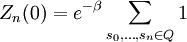
Another important related quantity is the topological pressure, defined as which will show up as the logarithm of the leading eigenvalue of the transfer operator of the solution. Free field solutionThe simplest model is the model where there is no interaction at all, and so V = 0 and Hn = 0. The partition function becomes If all states are allowed, that is, the underlying set of states is given by a full shift, then the sum may be trivially evaluated as
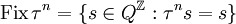
If neighboring spins are only allowed in certain specific configurations, then the state space is given by a subshift of finite type. The partition function may then be written as where card is the cardinality or count of a set, and Fix is the set of fixed points of the iterated shift function: The Interacting modelThe simplest case of the interacting model is the Ising model, where there the spin can only take on one of two values, This potential can be captured in a with the index The general solution for an arbitrary number of spins, and an arbitrary finite-range interaction, is given by the same general form. In this case, the precise expression for the matrix M is a bit more complex.
References
Categories: Statistical mechanics | Lattice models |
|
| This article is licensed under the GNU Free Documentation License. It uses material from the Wikipedia article "Potts_model". A list of authors is available in Wikipedia. |


 . Here,
 a continuous transition is observed, as in the Ising model where
  be a finite set of symbols, and let

 , acting as
![C_m[\xi_0, \ldots, \xi_k]= \{s \in Q^\mathbb{Z} : s_m = \xi_0, \ldots ,s_{m+k} = \xi_k \}](images/math/9/4/9/949f62c9610ae2356708523852e244b5.png)
 . Explicit representations for the cylinder sets can be gotten by noting that the string of values corresponds to a q-adic number, and thus, intuitively, the product topology resembles that of the real number line.
 on this topology. Any continuous function will do; for example
 , that is, an infinite string of spins. In the above example, the function V just picked out two spins out of the infinite string: the values
  as
as
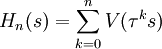
![[s_0, s_1, \ldots,s_n]](images/math/8/6/0/8603ebb50293e79956d30bd020f36747.png) of spins, plus the interaction energy of this set and all the other spins in the lattice. The
of spins, plus the interaction energy of this set and all the other spins in the lattice. The  limit of this function is the Hamiltonian of the system; for finite n, these are sometimes called the finite state Hamiltonians.
![Z_n(V) = \sum_{s_0,\ldots,s_n \in Q} \exp -\beta H_n(C_0[s_0,s_1,\ldots,s_n])](images/math/f/2/9/f29019908c300def39422fdba151302c.png)
![\mu (C_k[s_0,s_1,\ldots,s_n]) = \frac{1}{Z_n(V)} \exp -\beta H_n (C_k[s_0,s_1,\ldots,s_n])](images/math/e/4/0/e400de9cdb914c5b37d73badd48da721.png)
 . By endowing the configuration space with a probability measure built from a Hamiltonian in this way, the configuration space turns into a
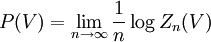

 matrix
  and only nearest neighbor spins interact. The interaction potential is given by
 matrix with matrix elements
 . The partition function is then given by