To use all functions of this page, please activate cookies in your browser.
My watch list
my.chemeurope.com
my.chemeurope.com
With an accout for my.chemeurope.com you can always see everything at a glance – and you can configure your own website and individual newsletter.
- My watch list
- My saved searches
- My saved topics
- My newsletter
Determination of equilibrium constantsEquilibrium constants are determined in order to quantify chemical equilibria. When an equilibrium constant is expressed as a concentration quotient, it is implied that the activity quotient is constant. In order for this assumption to be valid equilibrium constants should be determined in a medium of relatively high ionic strength. Where this is not possible, consideration should be given to possible activity variation. The equilibrium expression above is a function of the concentrations [A], [B] etc. of the chemical species in equilibrium. The equilibrium constant value can be determined if any one of these concentrations can be measured. The general procedure is that the concentration in question is measured for a series of solutions with known analytical concentrations of the reactants. Typically, a titration is performed with one or more reactants in the titration vessel and one or more reactants in the burette. Knowing the analytical concentrations of reactants initially in the reaction vessel and in the burette, all analytical concentrations can be derived as a function of the volume (or mass) of titrant added. The equilibrium constants may be derived by best-fitting of the experimental data with a chemical model of the equilibrium system. Product highlight
Experimental methodsThere are four main experimental methods. For less commonly used methods see Rossotti and Rossotti[1] Potentiometric measurementsA free concentration [A] or activity {A} is measured by means of an ion selective electrode such as the glass electrode. If the electrode is calibrated using activity standards it is assumed that the Nernst equation applies in the form
where E0 is the standard electrode potential. When buffer solutions of known pH are used for calibration the meter reading will be pH.
At 298K, 1 pH unit is approximately equal to 59 mV.[2] When the electrode is calibrated with solutions of known concentration, by means of a strong acid/strong base titration, for example, a modified Nernst equation is assumed.
s an empirical slope factor. A solution of known hydrogen ion concentration may be prepared by standardization of a strong acid against borax. Constant-boiling hydrochloric acid may also be used as a primary standard for hydrogen ion concentration. Spectrophotometric measurementsAbsorbanceIt is assumed that the Beer-Lambert law applies. where Fluorescence (luminescence) intensityIt is assumed that the scattered light intensity is a linear function of species’ concentrations. where φ is a proportionality constant. NMR chemical shift measurementsChemical exchange is assumed to be rapid on the NMR time-scale. An individual chemical shift Calorimetric measurementsSimultaneous measurement of K and ΔH for 1:1 adducts is routinely carried out using Isothermal Titration Calorimetry. Extension to more complex systems is limited by the availability of suitable software. Range and limitations
Computational methodsIt is assumed that the experimental data which have been collected comprise a set of data points. At each i'th data point, the analytical concentrations of the reactants, TA(i), TB(i) etc. are known along with a measured quantity, yi, that depends on one or more of these analytical concentrations. A general computational procedure has three main components.
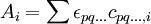
The chemical modelThe chemical model consists of a set of chemical species present in solution, both the reactants added to the reaction mixture and the complex species formed from them. Denoting the reactants by A, B ..., each complex species is specified by the stoichiometric coefficients that relate the particular combination of reactants forming them. When using general-purpose computer programs, it is usual to use cumulative, association constants, as shown above. When reactants and complexes are chemical species ionic charges should be shown explicitly. With aqueous solutions the concentrations of proton (hydronium ion) and hydroxide ion are constrained by the self-dissociation of water. With dilute solutions the concentration of water can be assumed to be constant so the equilibrium expression is written in the familiar form of the ionic product of water. When both H+ and OH− must be considered as reactants, one of them is eliminated from the model by specifying that its concentration is to be derived from the concentration of the other. Usually the concentration of the hydroxide ion is given by In this case the equilibrium constant for the formation of hydroxide has the stoichiometric coefficients -1 in regard to the proton and zero for the other reactants. This has important implications for all protonation equilibria in aqueous solution and for hydrolysis constants in particular. It is quite usual to omit from the model those species whose concentrations are considered to be negligible. For example it is usually assumed then there is no interaction between the reactants and/or complexes and the electrolyte used to maintain constant ionic strength or the buffer used to maintain constant pH. These assumptions may or may not be justified. Also, it is implicitly assumed that there are no other complex species present. When complexes are wrongly ignored a systematic error is introduced into the calculations. Equilibrium constant values are usually estimated initially by reference to data sources. Model selectionThis is the process whereby a variety of models are examined in order to find the model that best fits the experimental data, within experimental error. The main difficulty is with the so-called minor species. These are species whose concentration is so low that the effect on the measured quantity is at or below the level of error in the experimental measurement. The constant for a minor species may prove impossible to determine if there is no means to increase the concentration of the species. Speciation calculationsA speciation calculation is one in which the concentrations of all the species in an equilibrium system are calculated, knowing the analytical concentrations, TA, TB etc. of the reactants A, B etc. This means solving a set of non-linear equations of mass-balance
for the free concentrations [A], [B] etc. The concentrations of the complexes are derived from the free concentrations via the chemical model. Some authors[3][4] include the free reactant terms in the sums by declaring identity (unit) β constants for which the stoichiometric coefficients are 1 for the reactant concerned and zero for all other reactants: In this manner, all chemical species, including the free reactants, are treated in the same way, having been formed from the combination of reactants that is specified by the stoichiometric coefficients. The mass-balance equations assume the simpler form.
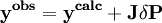
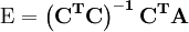
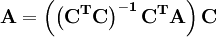
In a titration system the analytical concentrations of the reactants at each titration point are obtained from the inital conditions, the burette concentrations and volumes. The analytical (total) concentration of a reactant R at the i'th titration point is given by where R0 is the initial amount of R in the titration vessel, v0 is the initial volume, [R] is the concentration of R in the burette and vi is the volume added. The burette concentration of a reactant not present in the burette is taken to be zero. In general, solving these non-linear equations presents a formidable challenge because of the huge range over which the free concentrations may vary. At the beginning, values for the free concentrations must be estimated. Then, these values are refined, usually by means of Newton-Raphson iterations. The logarithms of the free concentrations may be refined rather than the free concentrations themselves. Refinement of the logarithms of the free concentrations has the added advantage of automatically imposing a non-negativity constraint on the free concentrations. Once the free reactant concentrations have been calculated, the concentrations of the complexes are derived from them and the equilibrium constants. Note that the free reactant concentrations can be regarded as implicit parameters in the equilibrium constant refinement process. In that context the values of the free concentrations are constrained by forcing the conditions of mass-balance to apply at all stages of the process. Equilibrium constant refinementThe objective of the refinement process it to find equilibrium constant values that give the best fit to the experimental data. This is usually achieved by minimising an objective function, U, by the method of non-linear least-squares. The matrix of weights, W, should be, ideally, the inverse of the variance-covariance matrix of the observations. It is rare for this to be known. However, when it is, the expectation value of U is one, which means that the data are fitted within experimental error. Most often only the diagonal elements are known, in which case the objective function simplifies to with Wi,j = 0 when j≠ i. Unit weights, Wi,i = 1, are often used but, in that case, the expectation value of U is the root mean square of the experimental errors. The minimization may be performed using the Gauss-Newton method with or without a Levenberg-Marquardt parameter. This method requires the elements of the Jacobian matrix, J, to be calculated. where Pk is the kth parameter of the refinement. One or more equilibrium constants may be parameters of the refinement. However, the measured quantities (see above) represented by y are not expressed in terms of the equilibrium constants, but in terms of the species concentrations, which are implicit functions of these parameters. Therefore the Jacobian elements must be obtained using implicit differentiation. Parameter increments δP are calculated by solving the normal equations, the first-order Taylor series gathered in matrix form as which are solved with where λ is the optional Marquardt parameter, I is the identity matrix, and the superscript T indicates the transpose of the matrix. The increments δP are added to the current parameter estimates to obtain better estimates, the species concentrations and ycalc values are recalculated at every data point and the procedure is repeated until no further reduction in U is achieved. A particular issue arises with NMR and spectrophotometric data. For the latter, the observed quantity is absorbance, A, and the Beer-Lambert law can be written as It can be seen that absorbance, A, is a linear function of the molar absorbptivities, ε, at the path length used. In matrix notation There are two approaches to the calculation of the unknown molar absorptivities
ImplementationsSome simple systems are amenable to spreadsheet calculations.[6] These calculations do not follow the general procedures outlined here and use SOLVER to perform the least-squares minimization. A large number of computer programs for equilibrium constant calculation have been published. See [7] for a bibliography. The most frequently used programs are:
References
|
|
| This article is licensed under the GNU Free Documentation License. It uses material from the Wikipedia article "Determination_of_equilibrium_constants". A list of authors is available in Wikipedia. |
![K=\frac{{[S]} ^\sigma {[T]}^\tau ... } {{[A]}^\alpha {[B]}^\beta ...}](images/math/2/9/6/296413eeef24f9a0f15328533924e416.png)


 is the optical path length,
 is the mole-fraction-weighted average of the shifts
![pA+qB...\rightleftharpoons A_pB_q...: \beta_{pq...}=\frac{[A_pB_q...]} {[A]^p[B]^q...}](images/math/3/b/f/3bf9fd93896854999b8a6c880e715d94.png)
![H_2O \rightleftharpoons H^+ + OH^-: K_W'=\frac{[H^+][OH^-]}{[H_2O]}](images/math/5/d/2/5d2a2f022d16fdf68d5d345f8387f351.png)
![K_W=[H^+][OH^-]\,](images/math/0/2/1/0219478cfab881ab94247dfecc4c691d.png)
![[OH^-]=K_W[H^+]^{-1}\,](images/math/a/6/3/a631af5ea88b765b4b2210d00b0434ec.png)
![T_A=[A]+\sum p\beta_{pq...}[A]^p[B]^q...](images/math/b/d/0/bd0b4edf7c368d76d3a5e255e5277fe7.png)
![T_B=[B]+\sum q\beta_{pq...}[A]^p[B]^q...](images/math/7/3/e/73ed067899476aad64ce4b62176e3f62.png)
![[A] = \beta_{10...}[A],[B] = \beta_{01...}[B] ...\,](images/math/7/4/9/74981762221b61c3a744ed00c43d5167.png)
![T_A=\sum p\beta_{pq...}[A]^p[B]^q...](images/math/d/5/3/d53a5abd5b8f39b99291ef6bb3c74f38.png)
![T_B=\sum q\beta_{pq...}[A]^p[B]^q...](images/math/2/b/b/2bbe6f511fab94fd428be00b7d999b6c.png)
![T_R=\frac{R_0+v_i[R]}{v_0+v_i}](images/math/2/a/0/2a095d4d36d46bb8a57561bb2d8ec3ad.png)


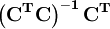 is an example of a pseudo-inverse.
Last viewed


