To use all functions of this page, please activate cookies in your browser.
My watch list
my.chemeurope.com
my.chemeurope.com
With an accout for my.chemeurope.com you can always see everything at a glance – and you can configure your own website and individual newsletter.
- My watch list
- My saved searches
- My saved topics
- My newsletter
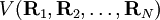
Molecular HamiltonianIn atomic, molecular, and optical physics as well as in quantum chemistry, molecular Hamiltonian is the name given to the Hamiltonian representing the energy of the electrons and nuclei in a molecule. This Hermitian operator and the associated Schrödinger equation play a central role in computational chemistry and physics for computing properties of molecules and aggregates of molecules, such as conductivity, optical, and magnetic properties, and reactivity. The bricks of the molecule are the nuclei, characterized by their atomic number Z, while the electrons, which have negative elementary charge -q, are its mortar. The charge of a nucleus is Zq. Electrons and nuclei are, to a very good approximation, point charges and point masses. The molecular Hamiltonian is a sum of several terms: its major terms are the kinetic energies of the electrons and the Coulomb (electrostatic) interactions between the two kinds of charged particles. The Hamiltonian that contains only the kinetic energies of electrons and nuclei, and the Coulomb interactions between them, is known as the Coulomb Hamiltonian. From it are missing a number of small terms, most of which are due to electronic and nuclear spin. Although it is generally assumed that the solution of the time-independent Schrödinger equation associated with the Coulomb Hamiltonian will predict most properties of the molecule, including its shape (three-dimensional structure), calculations based on the full Coulomb Hamiltonian are very scarce. The main reason being that its Schrödinger equation is very difficult to solve. Applications are restricted to small systems like the hydrogen molecule. Almost all calculations of molecular wavefunctions are based on the separation of the Coulomb Hamiltonian first devised by Born and Oppenheimer. The nuclear kinetic energy terms are omitted from the Coulomb Hamiltonian and one considers the remaining Hamiltonian as a Hamiltonian of electrons only. The stationary nuclei enter the problem only as generators of an electric potential in which the electrons move in a quantum mechanical way. Within this framework the molecular Hamiltonian has been simplified to the so-called clamped nucleus Hamiltonian, also called electronic Hamiltonian, that acts only on functions of the electronic coordinates. Once the Schrödinger equation of the clamped nucleus Hamiltonian has been solved for a sufficient number of constellations of the nuclei, an appropriate eigenvalue (usually the lowest) can be seen as a function of the nuclear coordinates, which leads to a potential energy surface. In practical calculations the surface is usually fitted in terms of some analytic functions. In the second step of the Born-Oppenheimer approximation the part of the full Coulomb Hamiltonian that depends on the electrons is replaced by the potential energy surface. This converts the total molecular Hamiltonian into another Hamiltonian that acts only on the nuclear coordinates. In the case of a breakdown of the Born-Oppenheimer approximation—which occurs when energies of different electronic states are close—the neighboring potential energy surfaces are needed, see this article for more details on this. The nuclear motion Schrödinger equation can be solved in a space-fixed (laboratory) frame, but then the translational and rotational (external) energies are not accounted for. Only the (internal) atomic vibrations enter the problem. Further, for molecules larger than triatomic ones, it is quite common to introduce the harmonic approximation, which approximates the potential energy surface as a quadratic function of the atomic displacements. This gives the harmonic nuclear motion Hamiltonian. Making the harmonic approximation, we can convert the Hamiltonian into a sum of uncoupled one-dimensional harmonic oscillator Hamiltonians. The one-dimensional harmonic oscillator is one of the few systems that allows an exact solution of the Schrödinger equation. Alternatively, the nuclear motion (rovibrational) Schrödinger equation can be solved in a special frame (an Eckart frame) that rotates and translates with the molecule. Formulated with respect to this body-fixed frame the Hamiltonian accounts for rotation, translation and vibration of the nuclei. Since Watson introduced in 1968 an important simplification to this Hamiltonian, it is often referred to as Watson's nuclear motion Hamiltonian, but it is also known as the Eckart Hamiltonian, Product highlight
Coulomb HamiltonianThe algebraic form of many observables—i.e., Hermitian operators representing observable quantities—is obtained by the following quantization rules:
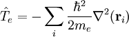
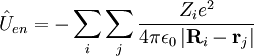
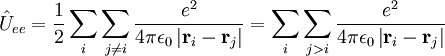
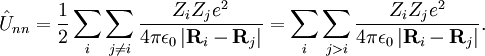
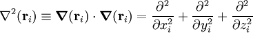
Classically the electrons and nuclei in a molecule have kinetic energy of the form p2/(2m) and interact via Coulomb interactions, which are inversely proportional to the distance rij between particle i and j. In this expression ri stands for the coordinate vector of any particle (electron or nucleus). But from here on we will reserve capital R to represent the nuclear coordinate, and lower case r for the electrons of the system. The coordinates can be taken to be expressed with respect to any Cartesian frame centered anywhere in space, because distance, being an inner product, is invariant under rotation of the frame and, being the norm of a difference vector, distance is invariant under translation of the frame as well. By quantizing the classical energy in Hamilton form one obtains the a molecular Hamilton operator that is often referred to as the Coulomb Hamiltonian. This Hamiltonian is a sum of 5 terms. They are
Here Mi is the mass of nucleus i, Zi is the atomic number of nucleus i, and me is the mass of the electron. The Laplace operator
of particle i is : Small termsIn the 1920s much spectroscopic evidence made it clear that the Coulomb Hamiltonian is missing certain terms. Especially for molecules containing heavier atoms, these terms, although much smaller than kinetic and Coulomb energies, are nonnegligible. These spectroscopic observations led to the introduction of a new degree of freedom for electrons and nuclei, namely spin. This empirical concept was given a theoretical basis by Dirac when he introduced a relativistically correct (Lorentz covariant) form of the one-particle Schrödinger equation. The Dirac equation predicts that spin and spatial motion of a particle interact via spin-orbit coupling. In analogy spin-other-orbit coupling was introduced. The fact that particle spin has some of the characteristics of a magnetic dipole led to spin-spin coupling. Further terms without a classical counterpart are the Fermi-contact term (interaction of electronic density on a finite size nucleus with the nucleus), and nuclear quadrupole coupling (interaction of a nuclear quadrupole with the gradient of an electric field due to the electrons). Finally a parity violating term predicted by the Standard Model must be mentioned. Although it is an extremely small interaction, it has attracted a fair amount of attention in the scientific literature because it gives different energies for the enantiomers in chiral molecules. The remaining part of this article will ignore spin terms and consider the solution of the eigenvalue (time-independent Schrödinger) equation of the Coulomb Hamiltonian. The Schrödinger equation of the Coulomb HamiltonianThe Coulomb Hamiltonian has a continuous spectrum due to to the center of mass motion of the molecule in homogeneous space. In classical mechanics it is easy to separate off the center of mass (COM) motion of a system of point masses. Classically the motion of the COM is uncoupled from the other motions. The COM moves uniformly (i.e., with constant velocity) through space as if it were a point particle with mass equal to the sum Mtot of the masses of all the particles. In quantum mechanics a free particle has as state function a plane wave function, which is a non-square-integrable function of well-defined momentum. The kinetic energy
of this particle covers Quantum mechanically the proper separation of the COM motion
is much more cumbersome than in classical mechanics. By introducing the coordinate vector The first term of H is the kinetic energy of the COM motion, which can be treated separately since H' does not depend on Not many actual molecular applications of H' exist, see, however, the seminal work[1] on the hydrogen molecule for an early application. In the great majority of computations of molecular wavefunctions the electronic problem is solved with the clamped nucleus Hamiltonian arising in the first step of the Born-Oppenheimer approximation. See Ref.[2] for a thorough discussion of the mathematical properties of the Coulomb Hamiltonian. Also it is discussed in this paper whether one can arrive a priori at the concept of a molecule (as a stable system of electrons and nuclei with a well-defined geometry) from the properties of the Coulomb Hamiltonian alone.
Clamped nucleus HamiltonianThe clamped nucleus Hamiltonian describes the energy of the electrons in the electrostatic field of the nuclei, where the nuclei are assumed to be stationary with respect to an inertial frame. The form of the electronic Hamiltonian is The coordinates of electrons and nuclei are expressed with respect to a frame that moves with the nuclei, so that the nuclei are at rest with respect to this frame. The frame stays parallel to a space-fixed frame. It is an inertial frame because the nuclei are assumed not to be accelerated by external forces or torques. The origin of the frame is arbitrary, it is usually positioned on a central nucleus or in the nuclear center of mass. Sometimes it is stated that the nuclei are "at rest in a space-fixed frame". This statement implies that the nuclei are viewed as classical particles, because a quantum mechanical particle cannot be at rest. (It would mean that it had simultaneously zero momentum and well-defined position, which contradicts Heisenberg's uncertainty principle). Since the nuclear positions are constants, the electronic kinetic energy operator is invariant under translation over any nuclear vector. The Coulomb potential, depending on difference vectors, is invariant as well. In the description of atomic orbitals and the computation of integrals over atomic orbitals this invariance is used by equipping all atoms in the molecule with their own localized frames parallel to the space-fixed frame. As explained in the article on the Born-Oppenheimer approximation, a sufficient number of solutions
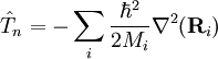
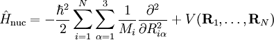
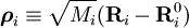
of the Schrödinger equation of Hel leads to a potential energy surface (PES) for where t and s are arbitrary vectors and Δφ is an infinitesimal angle, Δφ >> Δφ2. This invariance condition on the PES is automatically fulfilled when the PES is expressed in terms of differences of, and angles between, the Ri, which is usually the case. Harmonic nuclear motion HamiltonianIn the remaining part of this article we assume that the molecule is semi-rigid. In the second step of the BO approximation the nuclear kinetic energy Tn is reintroduced and the Schrödinger equation with Hamiltonian is considered. One would like to recognize in its solution: the motion of the nuclear center of mass (3 degrees of freedom), the overall rotation of the molecule (3 degrees of freedom), and the nuclear vibrations. In general, this is not possible with the given nuclear kinetic energy, because it does not separate explicitly the 6 external degrees of freedom (overall translation and rotation) from the 3N-6 internal degrees of freedom. In fact, the kinetic energy operator here is defined with respect to a space-fixed (SF) frame. If we were to move the origin of the SF frame to the nuclear center of mass, then, by application of the chain rule, nuclear mass polarization terms would appear. It is customary to ignore these terms altogether and we will follow this custom. In order to achieve a separation we must distinguish internal and external coordinates, to which end Eckart introduced conditions to be satisfied by the coordinates. We will show how these conditions arise in a natural way from a harmonic analysis in mass-weighted Cartesian coordinates. In order to simplify the expression for the kinetic energy we introduce mass-weighted displacement coordinates
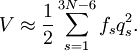
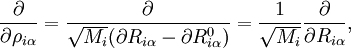
Since the kinetic energy operator becomes, If we make a Taylor expansion of V around the equilibrium geometry, and truncate after three terms (the so-called harmonic approximation), we can describe V with only the third term. The term V0 can be absorbed in the energy (gives a new zero of energy). The second term is vanishing because of the equilibrium condition. The remaining term contains the Hessian matrix F of V, which is symmetric and may be diagonalized with an orthogonal 3N x 3N matrix with constant elements: It can be shown from the invariance of V under rotation and translation that six of the eigenvectors of F (last six rows of Q) have eigenvalue zero (are zero-frequency modes). They span the external space. The first 3N-6 rows of Q are—for molecules in their ground state—eigenvectors with non-zero eigenvalue; they are the internal coordinates and form an orthonormal basis for a 3N - 6 dimensional subspace of the nuclear configuration space R3N, the internal space. The zero-frequency eigenvectors are orthogonal to the eigenvectors of non-zero frequency. It can be shown that these orthogonalities are in fact the Eckart conditions. The kinetic energy expressed in the internal coordinates is the internal (vibrational) kinetic energy. With the introduction of normal coordinates the vibrational (internal) part of the Hamiltonian for the nuclear motion becomes in the harmonic approximation The corresponding Schrödinger equation is easily solved, it factorizes into 3N-6 equations for one-dimensional harmonic oscillators. The main effort in this approximate solution of the nuclear motion Schrödinger equation is the computation of the Hessian F of V and its diagonalization. This approximation to the nuclear motion problem, described in 3N mass-weighted Cartesian coordinates, became standard in quantum chemistry, since the days (1980s-1990s) that algorithms for accurate computations of the Hessian F became available. Apart from the harmonic approximation, it has as a further deficiency that the external (rotational and translational) motions of the molecule are not accounted for. They are accounted for in a rovibrational Hamiltonian that sometimes is called Watson's Hamiltonian. Watson's nuclear motion HamiltonianIn order to obtain a Hamiltonian for external (translation and rotation) motions coupled to the internal (vibrational) motions, it is common to return at this point to classical mechanics and to formulate the classical kinetic energy corresponding to these motions of the nuclei. Classically it is easy to separate the translational—center of mass—motion from the other motions. However, the separation of the rotational from the vibrational motion is more difficult and is not completely possible. This ro-vibrational separation was first achieved by Eckart[3] in 1935 by imposing by what is now known as Eckart conditions. Since the problem is described in a frame (an "Eckart" frame) that rotates with the molecule, and hence is a non-inertial frame, energies associated with the fictitious forces: centrifugal and Coriolis force appear in the kinetic energy. In general, the classical kinetic energy T defines the metric tensor g = (gij) associated with the curvilinear coordinates s = (si) through
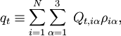
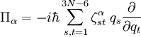
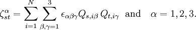
The quantization step is the transformation of this classical kinetic energy into a quantum mechanical operator. It is common to follow Podolsky[4] by writing down the Laplace-Beltrami operator in the same (generalized, curvilinear) coordinates s as used for the classical form. The equation for this operator requires the inverse of the metric tensor g and its determinant. Multiplication of the Laplace-Beltrami operator by The nuclear motion Hamiltonian was obtained by Wilson and Howard in 1936, [5] who followed this procedure, and further refined by Darling and Dennison in 1940.[6] It remained the standard until 1968, when Watson[7] was able to simplify it drastically by commuting through the derivatives the determinant of the metric tensor. We will give the ro-vibrational Hamiltonian obtained by Watson, which often is referred to as the Watson Hamiltonian. Before we do this we must mention that a derivation of this Hamiltonian is also possible by starting from the Laplace operator in Cartesian form, application of coordinate transformations, and use of the chain rule.[8] The Watson Hamiltonian, describing all motions of the N nuclei, is The first term is the center of mass term The second term is the rotational term akin to the kinetic energy of the rigid rotor. Here
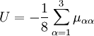
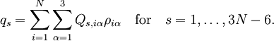
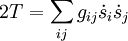
with the Coriolis coupling constant: Here εαβγ is the Levi-Civita symbol. The terms quadratic in the The potential-like term U is the Watson term: proportional to the trace of the effective reciprocal inertia tensor. The fourth term in the Watson Hamiltonian is the kinetic energy associated with the vibrations of the atoms (nuclei) expressed in normal coordinates qs, which as stated above, are given in terms of nuclear displacements ρiα by Finally V is the unexpanded potential energy by definition depending on internal coordinates only. In the harmonic approximation it takes the form References
Further reading
See also
Categories: Molecular physics | Quantum chemistry | Spectroscopy |
|
| This article is licensed under the GNU Free Documentation License. It uses material from the Wikipedia article "Molecular_Hamiltonian". A list of authors is available in Wikipedia. |


 and interpret q as a multiplicative operator. Here
  is the nabla operator, a vector operator consisting of first derivatives. The well-known commutation relations for the p and q operators follow directly from the differentiation rules.

 . Since the kinetic energy operator is an inner product, it is invariant under rotation of the Cartesian frame with respect to which xi, yi, and zi are expressed. The kinetic energy operator, however, is not invariant under translation (choice of origin of the frame).
 . The position of the COM is uniformly probable everywhere, in agreement with the Heisenberg uncertainty principle.
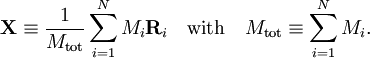
 of the center of mass as three of the degrees of freedom of the system and eliminating the coordinate vector of one (arbitrary) particle, so that the number of degrees of freedom stays the same, one obtains by a linear transformation a new set of coordinates ti. These coordinates are linear combinations of the old coordinates of all particles (nuclei and electrons). By applying the chain rule one can show that

 consists of the Coulomb terms expressed in the new coordinates. The first term of
 . It is assumed that the functional dependence of V on its coordinates is such that


 .
.
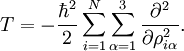


![\hat{H}_\mathrm{nuc} \approx \frac{1}{2} \sum_{t=1}^{3N-6} \left[-\hbar^2 \frac{\partial^2}{\partial q_{t}^2} + f_t q_t^2 \right] .](images/math/3/0/d/30d9b5a62d763b4596dbd352549bef55.png)
 .
.
 gives the required quantum mechanical kinetic energy operator. When we apply this recipe to Cartesian coordinates, which have unit metric, the same kinetic energy is obtained as by application of the quantization rules.

 is the α component of the body-fixed rigid rotor angular momentum operator,
see this article for its expression in terms of Euler angles. The operator
is the α component of the body-fixed rigid rotor angular momentum operator,
see this article for its expression in terms of Euler angles. The operator  is a component of an operator known
as the vibrational angular momentum operator (although it does not satisfy angular momentum commutation relations),
is a component of an operator known
as the vibrational angular momentum operator (although it does not satisfy angular momentum commutation relations),
 are Coriolis terms.
The quantities Q s, iγ are the components of the normal coordinates introduced above.
Alternatively, normal coordinates may be obtained by application of Wilson's
are Coriolis terms.
The quantities Q s, iγ are the components of the normal coordinates introduced above.
Alternatively, normal coordinates may be obtained by application of Wilson's  is called the effective reciprocal inertia tensor. If all q s were zero (rigid molecule) the Eckart frame would coincide with a principal axes frame (see