To use all functions of this page, please activate cookies in your browser.
My watch list
my.chemeurope.com
my.chemeurope.com
With an accout for my.chemeurope.com you can always see everything at a glance – and you can configure your own website and individual newsletter.
- My watch list
- My saved searches
- My saved topics
- My newsletter
Dirac equation
In physics, the Dirac equation is a relativistic quantum mechanical wave equation formulated by British physicist Paul Dirac in 1928 and provides a description of elementary spin-½ particles, such as electrons, consistent with both the principles of quantum mechanics and the theory of special relativity. The equation demands the existence of antiparticles and actually predated their experimental discovery, making the discovery of the positron, the antiparticle of the electron, one of the greatest triumphs of modern theoretical physics. Product highlight
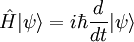
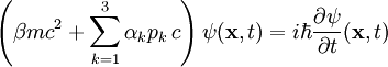
Mathematical formulationThe Dirac equation in the form originally proposed by Dirac is:
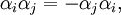
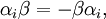
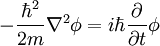
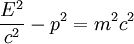
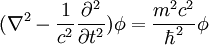
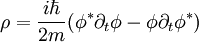
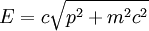
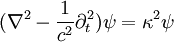
The new elements in this equation are the 4x4 matrices αk and β, and the four-component wavefunction ψ. The matrices are all Hermitian and have squares equal to the identity matrix, and they all mutually anticommute: where i and j are distinct and range from 1 to 3. These matrices, and the form of the wavefunction, have a deep mathematical significance. The algebraic structure represented by the Dirac matrices had been created some 50 years earlier by the English mathematician W. K. Clifford, which in turn had been based on the mid-19th century work of the German mathematician Hermann Grassmann in his "Lineare Ausdehnungslehre" (Theory of Linear Extensions). The latter had been regarded as well-nigh incomprehensible by most of his contemporaries. The appearance of something so seemingly abstract, at such a late date, in such a direct physical manner, amounts to one of the most remarkable chapters in the history of physics. Comparison with the Schrödinger equationThe Dirac equation is superficially similar to the Schrödinger equation for a free mass: The left side represents the square of the momentum operator divided by twice the mass, which, classically speaking, is the kinetic energy. If one wants to get a relativistic generalization of this equation, then the space and time derivatives must enter symmetrically, as they do in the Maxwell theory of the electromagnetic field, which is known to be relativistically invariant - that is, the derivatives must be of the same order in space and time. Now, in relativity, the momentum and the energy are each part of an invariant object, the 4-momentum, and they are connected by the relativistically invariant relation with m now representing the rest mass. If we replace E and p by their operator equivalents in the Schrödinger theory, we get a differential equation that is a valid relativistic generalization of the Schrödinger equation: where it is assumed that the wave function is now a relativistic scalar. In fact Schrödinger, who was well acquainted with relativity, tried this equation before the one that bears his name, but found it unsuitable. Because the time derivative is second order, one must specify both the initial value of There was an even more serious objection to be raised - in the Schrödinger theory, the probability density is given by the positive definite expression
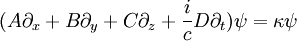
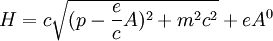
and its current by with the conservation of probability density expressed as In a relativistic theory, the form of the probability density must match that of the current when we replace Everything is now perfectly relativistic, but the probability density is not positive definite, because one may freely choose the initial values of both φ and Dirac's coupWhat is needed, then, is an equation that is first-order in both space and time. One could formally take the relativistic expression for the energy As the story goes, Dirac was staring into the fireplace at Cambridge, pondering this problem, when he hit upon the idea of taking the square root of the wave operator thus: On multiplying out the right side, we see that in order to get all the cross-terms such as
with
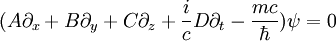
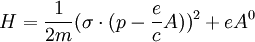
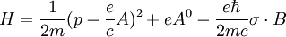
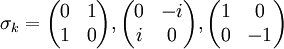
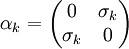
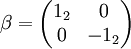
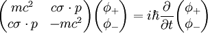
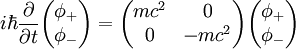
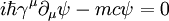
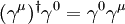
Dirac, who had just then been intensely involved with working out the foundations of Heisenberg's matrix mechanics, immediately understood that these conditions could be met if A, B... are matrices, with the implication that the wave function has multiple components. This immediately explained the appearance of two-component wave functions in Pauli's phenomenological theory of spin, something that up until then had been regarded as mysterious, even to Pauli himself. However, one needs at least 4x4 matrices to set up a system with the properties desired - so the wave function had four components, not two, as in the Pauli theory. Given the factorization in terms of these matrices, one can now write down immediately an equation with κ to be determined. Applying again the matrix operator on either side yields On taking With (A,B,C) = iβαk and D = β, we get the Dirac equation. Comparison with the Pauli theoryThe necessity of introducing half-integral spin goes back experimentally to the results of the Stern-Gerlach experiment. A beam of atoms is run through a strong inhomogeneous magnetic field, which then splits into N parts depending on the intrinsic angular momentum of the atoms. It was found that for silver atoms, the beam was split in two - the ground state therefore could not be integral, because even if the intrinsic angular momentum of the atoms were as small as possible, 1, the beam would be split into 3 parts, corresponding to atoms with Lz = -1, 0, and +1. The conclusion is that silver atoms have net intrinsic angular momentum of 1/2. Pauli set up a theory which explained this splitting by introducing a two-component wave function and a corresponding correction term in the Hamiltonian, representing a semi-classical coupling of this wave function to an applied magnetic field, as so: Here Aμ is the applied electromagnetic field, and the three sigmas are Pauli matrices. e is the charge of the particle, e.g. e = − e0 for the electron. On squaring out the first term, a residual interaction with the magnetic field is found, along with the usual Hamiltonian of a charged particle interacting with an applied field: This Hamiltonian is now a 2x2 matrix, so the Schrödinger equation based on it, must use a two-component wave function. Pauli had introduced the sigma matrices as pure phenomenology - Dirac now had a theoretical argument that implied that spin was somehow the consequence of the marriage of quantum theory to relativity. The Pauli matrices share the same properties as the Dirac matrices - they are all Hermitian, square to 1, and anticommute. This allows one to immediately find a representation of the Dirac matrices in terms of the Pauli matrices: The Dirac equation now may be written as an equation coupling two-component spinors: Notice that on the diagonal we find the rest energy of the particle. If we set the momentum to zero - that is, bring the particle to rest - then we have The equations for the individual two-spinors are now decoupled, and we see that the "top" and "bottom" two-spinors are individually eigenfunctions of the energy with eigenvalues equal to plus and minus the rest energy, respectively. The appearance of this negative energy eigenvalue is completely consistent with relativity. It should be strongly emphasized that this separation in the rest frame is not an invariant statement - the "bottom" two-spinor does not represent antimatter as such in general. The entire four-component spinor represents an irreducible whole - in general, states will have an admixture of positive and negative energy components. If we couple the Dirac equation to an electromagnetic field, as in the Pauli theory, then the positive and negative energy parts will be mixed together, even if they are originally decoupled. Dirac's main problem was to find a consistent interpretation of this mixing. As we shall see below, it brings a new phenomenon into physics - matter/antimatter creation and annihilation. Covariant form and relativistic invarianceThe covariant form of the Dirac equation is (employing the Einstein summation convention) In the above, γ0 is Hermitian, and the γk are anti-Hermitian, with the definition
This may be summarized using the Minkowski metric on spacetime in the form
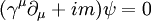
where the bracket expression {a, b} means ab + ba, the anticommutator. These are the defining relations of a Clifford algebra over a pseudo-orthogonal 4-d space with metric signature (+---). Note that one may also employ the metric form (-+++) by multiplying all the gammas by a factor of i. At an elementary level, the choice may be regarded as conventional, but there are specific reasons for preferring the former, both mathematically and for convenience in calculation and physical interpretation. In the literature, one almost always finds the convention (+---) in use. The specific Clifford algebra employed in the Dirac equation is known as the Dirac algebra. The Dirac equation may be interpreted as an eigenvalue expression, where the rest mass is proportional to an eigenvalue of the 4-momentum operator, the proportion being the speed of light in vacuo:
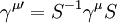
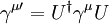
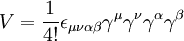
In practice, physicists often use units of measure such that A fundamental theorem states that if two distinct sets of matrices are given that both satisfy the Clifford relations, then they are connected to each other by a similarity transformation: If in addition the matrices are all unitary, as are the Dirac set, then S itself is unitary; The transformation U is unique up to a multiplicative factor of absolute value 1. Let us now imagine a Lorentz transformation to have been performed on the derivative operators, which form a covariant vector. In order that the operator If we now define the transformed spinor then we have the transformed Dirac equation Thus, once we settle on a unitary representation of the gammas, it is final providing we transform the spinor according the unitary transformation that corresponds to the given Lorentz transformation. These considerations reveal the origin of the gammas in geometry, hearkening back to Grassmann's original motivation - they represent a fixed basis of unit vectors in spacetime. Similarly, products of the gammas such as γμγν represent oriented surface elements, and so on. With this in mind, we can find the form the unit volume element on spacetime in terms of the gammas as follows. By definition, it is In order that this be an invariant, the epsilon symbol must be a tensor, and so must contain a factor of
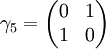
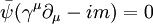
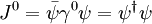
This matrix is given the special symbol γ5, owing to its importance when one is considering improper transformations of spacetime, that is, those that change the orientation of the basis vectors. In the representation we are using for the gammas, it is Also note that could as easily have taken the negative square root of the determinant of g - the choice amounts to an initial handedness convention. Adjoint equation and Dirac currentBy defining the adjoint spinor and noticing that
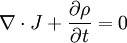
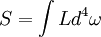
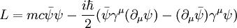
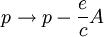
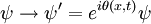
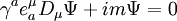
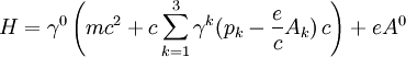
we obtain, by taking the Hermitian conjugate of the Dirac equation and multiplying from the right by γ0, the adjoint equation: where Now we see the great advantage of the first-order equation over the one Schrödinger had tried - this is the conserved probability current density required by relativistic invariance, only now its 0-component is positive definite: The Dirac equation and its adjoint are the Euler-Lagrange equations of the 4-d invariant action integral where the scalar L is the Dirac Lagrangian and for the purposes of variation, ψ and Coupling to an electromagnetic fieldTo consider problems in which an applied electromagnetic field interacts with the particles described by the Dirac equation, one uses the correspondence principle, and takes over into the theory the corresponding expression from classical mechanics, whereby the total momentum of a charged particle in an external field is modified as so: In natural units, the Dirac equation then takes the form This validity of this prescription is confirmed experimentally with great precision. It is known as minimal coupling, and is found throughout particle physics. Indeed, while the introduction of the electromagnetic field in this way is essentially phenomenological in this context, it rises to a fundamental principle in quantum field theory. Now as stated above, the transformation U is defined only up to a phase factor eiθ. Also, the fundamental observable of the Dirac theory, the current, is unchanged if we multiply the wave function by an arbitrary phase. We may exploit this to get the form of the mutual interaction of a Dirac particle and the electromagnetic field, as opposed to simply considering a Dirac particle in an applied field, by assuming this arbitrary phase factor to depend continuously on position: Notice now that In order to preserve minimal coupling, we must add to the potential a term proportional to the gradient of the phase. But we know from electrodynamics that this leaves the electromagnetic field itself invariant. The value of the phase is arbitrary, but not how it changes from place to place. This is the starting point of gauge theory, which is the main principle on which quantum field theory is based. The simplest such theory, and the one most thoroughly understood, is known as quantum electrodynamics. The equations of field theory thus have invariance under both Lorentz transformations and gauge transformations. Curved spacetime Dirac equationDirac equation can be written in curved spacetime using vierbein fields. Vierbeins describe a local frame that enables to define Dirac matrices at every point. Contracting these matrices with vierbeins give the right transformation properties. This way Dirac equation takes the following form in curved spacetime [1]: Here where ηac is the Lorentzian metric, σab is the commutator of Dirac matrices: and where Physical interpretationThe Dirac theory, while providing a wealth of information that is accurately confirmed by experiments, nevertheless introduces a new physical paradigm that appears at first difficult to interpret and even paradoxical. Some of these issues of interpretation must be regarded as open questions. Here we will see how the Dirac theory brilliantly answered some of the outstanding issues in physics at the time it was put forward, while posing others that are still the subject of debate. Identification of observablesThe critical physical question in a quantum theory is - what are the physically observable quantities defined by the theory? According to general principles, such quantities are defined by Hermitian operators that act on the Hilbert space of possible states of a system. The eigenvalues of these operators are then the possible results of measuring the corresponding physical quantity. In the Schrödinger theory, the simplest such object is the overall Hamiltonian, which represents the total energy of the system. If we wish to maintain this interpretation on passing to the Dirac theory, we must take the Hamiltonian to be This looks promising, because we see by inspection the rest energy of the particle and, in case A = 0, the energy of a charge placed in an electric potential eA0. What about the term involving the vector potential? In classical electrodynamics, the energy of a charge moving in an applied potential is Thus the Dirac Hamiltonian is fundamentally distinguished from its classical counterpart, and we must take great care to correctly identify what is an observable in this theory. Much of the apparent paradoxical behavior implied by the Dirac equation amounts to a misidentification of these observables. Let us now describe one such effect. (cont'd) HistorySince the Dirac equation was originally invented to describe the electron, we will generally speak of "electrons" in this article. The equation also applies to quarks, which are also elementary spin-½ particles. A modified Dirac equation can be used to approximately describe protons and neutrons, which are not elementary particles (they are made up of quarks), but have a net spin of ½. Another modification of the Dirac equation, called the Majorana equation, is thought to describe neutrinos — also spin-½ particles. The Dirac equation describes the probability amplitudes for a single electron. This is a single-particle theory; in other words, it does not account for the creation and destruction of the particles. It gives a good prediction of the magnetic moment of the electron and explains much of the fine structure observed in atomic spectral lines. It also explains the spin of the electron. Two of the four solutions of the equation correspond to the two spin states of the electron. The other two solutions make the peculiar prediction that there exist an infinite set of quantum states in which the electron possesses negative energy. This strange result led Dirac to predict, via a remarkable hypothesis known as "hole theory," the existence of particles behaving like positively-charged electrons. Dirac thought at first these particles might be protons. He was chagrined when the strict prediction of his equation (which actually specifies particles of the same mass as the electron) was verified by the discovery of the positron in 1932. When asked later why he hadn't actually boldly predicted the yet unfound positron with its correct mass, Dirac answered "Pure cowardice!" He shared the Nobel Prize anyway, in 1933. Despite these successes, Dirac's theory is flawed by its neglect of the possibility of creating and destroying particles, one of the basic consequences of relativity. This difficulty is resolved by reformulating it as a quantum field theory. Adding a quantized electromagnetic field to this theory leads to the theory of quantum electrodynamics (QED). Moreover the equation cannot fully account for particles of negative energy but is restricted to positive energy particles. A similar equation for spin 3/2 particles is called the Rarita-Schwinger equation. Hole theoryThe negative E solutions found in the preceding section are problematic, for it was assumed that the particle has a positive energy. Mathematically speaking, however, there seems to be no reason for us to reject the negative-energy solutions. Since they exist, we cannot simply ignore them, for once we include the interaction between the electron and the electromagnetic field, any electron placed in a positive-energy eigenstate would decay into negative-energy eigenstates of successively lower energy by emitting excess energy in the form of photons. Real electrons obviously do not behave in this way. To cope with this problem, Dirac introduced the hypothesis, known as hole theory, that the vacuum is the many-body quantum state in which all the negative-energy electron eigenstates are occupied. This description of the vacuum as a "sea" of electrons is called the Dirac sea. Since the Pauli exclusion principle forbids electrons from occupying the same state, any additional electron would be forced to occupy a positive-energy eigenstate, and positive-energy electrons would be forbidden from decaying into negative-energy eigenstates. Dirac further reasoned that if the negative-energy eigenstates are incompletely filled, each unoccupied eigenstate – called a hole – would behave like a positively charged particle. The hole possesses a positive energy, since energy is required to create a particle–hole pair from the vacuum. As noted above, Dirac initially thought that the hole might be the proton, but Hermann Weyl pointed out that the hole should behave as if it had the same mass as an electron, whereas the proton is over 1800 times heavier. The hole was eventually identified as the positron, experimentally discovered by Carl Anderson in 1932. It is not entirely satisfactory to describe the "vacuum" using an infinite sea of negative-energy electrons. The infinitely negative contributions from the sea of negative-energy electrons has to be canceled by an infinite positive "bare" energy and the contribution to the charge density and current coming from the sea of negative-energy electrons is exactly canceled by an infinite positive "jellium" background so that the net electric charge density of the vacuum is zero. In quantum field theory, a Bogoliubov transformation on the creation and annihilation operators (turning an occupied negative-energy electron state into an unoccupied positive energy positron state and an unoccupied negative-energy electron state into an occupied positive energy positron state) allows us to bypass the Dirac sea formalism even though, formally, it is equivalent to it. In certain applications of condensed matter physics, however, the underlying concepts of "hole theory" are valid. The sea of conduction electrons in an electrical conductor, called a Fermi sea, contains electrons with energies up to the chemical potential of the system. An unfilled state in the Fermi sea behaves like a positively-charged electron, though it is referred to as a "hole" rather than a "positron". The negative charge of the Fermi sea is balanced by the positively-charged ionic lattice of the material. Dirac bilinearsThere are five different (neutral) Dirac bilinear terms not involving any derivatives:
where A Dirac mass term is an S coupling. A Yukawa coupling may be S or P. The electromagnetic coupling is V. The weak interactions are V-A. See also
References
Selected papers
Textbooks
|
|||||||||||||||||||||||||
| This article is licensed under the GNU Free Documentation License. It uses material from the Wikipedia article "Dirac_equation". A list of authors is available in Wikipedia. |


 is the reduced Planck's constant,
 as well as
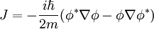
 by
by  , and in order that the conservation of probability current be a relativistically invariant expression, must form the 0-component of a 4-vector - thus we must have
 , replace p by its operator equivalent, expand the square root in an infinite series of derivative operators, set up an eigenvalue problem, then solve the equation formally by iterations. Most physicists had little faith in such a process, even if it were technically possible.

 to vanish, we must assume
 we find that all the components of the wave function individually satisfy the relativistic energy-momentum relation. Thus the sought-for equation that is first-order in both space and time is

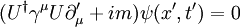
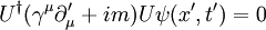
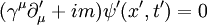
 remain invariant, the gammas must transform among themselves as a contravariant vector with respect to their spacetime index. These new gammas will themselves satisfy the Clifford relations, because of the orthogonality of the Lorentz transformation. By the fundamental theorem, we may replace the new set by the old set subject to a unitary transformation. In the new frame, remembering that the rest mass is a relativistic scalar, the Dirac equation will then take the form

 , where g is the determinant of the metric tensor. Since this is negative, that factor is imaginary. Thus

 ,
,
 is understood to act to the left. Multiplying the Dirac equation by
  from the left, and the adjoint equation by
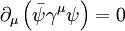


 is the vierbein and
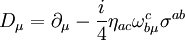
![\sigma^{ab}=\frac{i}{2} \left[\gamma^{a},\gamma^{b}\right]](images/math/8/1/2/812d0e8c943b37ea6e2ffef732f5f54c.png)
 is the spin connection:
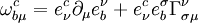
 is the Christoffel symbol. Note that here, Latin letters denote the "Lorentzian" indeces and Greek ones denote "Riemannian" indices.
 (scalar, P-even)
 (scalar, P-odd)
 (vector, P-even)
 (vector, P-odd)
 (antisymmetric tensor, P-even),
![\sigma^{\mu\nu}=\frac{i}{2} \left[\gamma^{\mu},\gamma^{\nu}\right]](images/math/9/1/a/91ace9245feb625bea96bf7446decf84.png) and
and 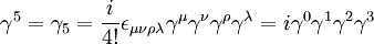 .
.


