My watch list

Primitive equations

The primitive equations are a version of the Navier-Stokes equations that describe hydrodynamical flow on the sphere under the assumptions that vertical motion is much smaller than horizontal motion (hydrostasis) and that the fluid layer depth is small compared to the radius of the sphere. Thus, they are a good approximation of global atmospheric flow and are used in most atmospheric models. The primitive equations may be linearized to yield Laplace's tidal equations, an eigenvalue problem from which the analytical solution to the latitudinal structure of the flow may be determined.

In general, nearly all forms of the primitive equations relate the five variables (u,v,ω,T,φ), and their evolution over space and time.

The equations were first written down by Vilhelm Bjerknes.^[1]

Additional recommended knowledge

Don't let static charges disrupt your weighing accuracy

Safe Weighing Range Ensures Accurate Results

How to ensure accurate weighing results every day?

1 Definitions
2 Forces that cause atmospheric motion
3 Forms of the primitive equations
- 3.1 Vertical pressure, cartesian tangential plane
- 3.2 Primitive equations using sigma coordinate system, polar stereographic projection
4 Solution to the primitive equations
- 4.1 Forecasting temperature
- 4.2 Forecasting precipitable water and pressure thickness
5 References
6 See also

Definitions

$u$ is the zonal velocity (velocity in the east/west direction tangent to the sphere).
$v$ is the meridional velocity (velocity in the north/south direction tangent to the sphere).
$ω$ is the vertical velocity
$T$ is the temperature
$φ$ is the geopotential
$f$ is the term corresponding to the Coriolis force, and is equal to $2Ω s i n (φ)$ , where $Ω$ is the angular rotation rate of the Earth ( $2π / 24$ radians per hour), and $φ$ is the latitude.
$R$ is the gas constant
$p$ is the pressure
$c p$ is the specific heat
$J$ is the heat flow per unit time per unit mass
$π$ is the exner function
$θ$ is the potential temperature

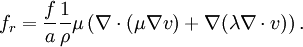
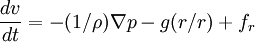
Forces that cause atmospheric motion

Forces that cause atmospheric motion include the pressure gradient force, force of gravitation, and friction. Together, they created the forces that accelerate our atmosphere.

The pressure gradient force can be written as

$\frac{f}{m} = \frac{1}{\rho} \frac{dp}{dx}.$

Gravitational force accelerates objects at approximately 9.81 m/s² directly toward the center of the Earth.

The frictional force can be approximated as

$f_r = {f \over a} {1 \over \rho} \mu\left(\nabla\cdot(\mu \nabla v) + \nabla(\lambda\nabla\cdot v) \right).$

Using Newton's second law, these forces (referenced in the equations above as the accelerations due to these forces) may be summed to produce an equation of motion that describes this system. This equation can be written in the form:

$\frac{dv}{dt} = - (1/\rho) \nabla p - g(r/r) + f_{r}$

g = g e

Therefore, to complete the system of equations and obtain 6 equations and 6 variables:

$\frac{dv}{dt} = - (1/\rho)\nabla p - g(r/r) + (1/\rho)\left[\nabla\cdot (\mu \nabla v) + \nabla(\lambda \nabla\cdot v)\right]$
$c_{v} \frac{dT}{dt} + p \frac{d\alpha}{dt} = q + f$
$\frac{dp}{dx} + \rho\nabla\cdot v = 0$
$p = ρ R T$

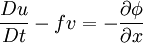
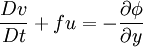
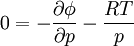
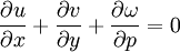
Forms of the primitive equations

The precise form of the primitive equations depends on the vertical coordinate system chosen, such as pressure coordinates, log pressure coordinates, or sigma coordinates. Furthermore, the velocity, temperature, and geopotential variables may be decomposed into mean and perturbation components using Reynolds decomposition.

Vertical pressure, cartesian tangential plane

In this form pressure is selected as the vertical coordinate and the horizontal coordinates are written for the cartesian tangential plane (i.e. a plane tangent to some point on the surface of the Earth). This form does not take the curvature of the Earth into account, but is useful for visualizing some of the physical processes involved in formulating the equations due to its relative simplicity.

Note that the capital derivatives are the material derivatives.

the geostrophic momentum equations

$\frac{Du}{Dt} - f v = -\frac{\partial \phi}{\partial x}$

$\frac{Dv}{Dt} + f u = -\frac{\partial \phi}{\partial y}$

the hydrostatic equation, a special case of the vertical momentum equation in which there is no background vertical acceleration.

$0 = -\frac{\partial \phi}{\partial p} - \frac{R T}{p}$

the continuity equation, connecting horizontal divergence/convergence to vertical motion under the hydrostatic approximation ( $d p = - ρ d φ$ ):

$\frac{\partial u}{\partial x} + \frac{\partial v}{\partial y} + \frac{\partial \omega}{\partial p} = 0$

and the thermodynamic energy equation, a consequence of the first law of thermodynamics

$\frac{\partial T}{\partial t} + u \frac{\partial T}{\partial x} + v \frac{\partial T}{\partial y} + \omega \left( \frac{\partial T}{\partial p} + \frac{R T}{p c_p} \right) = \frac{J}{c_p}$

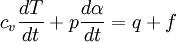
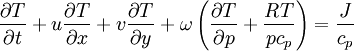
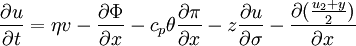
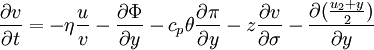
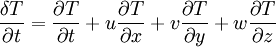
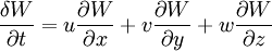
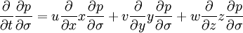
When a statement of the conservation of water vapor substance is included, these six equations form the basis for any numerical weather prediction scheme.

Primitive equations using sigma coordinate system, polar stereographic projection

According to the National Weather Service Handbook No. 1 - Facsimile Products, the primitive equations can be simplified into the following equations:

Zonal wind:

$\frac{\partial u}{\partial t} = \eta v - \frac{\partial \Phi}{\partial x} - c_p \theta \frac{\partial \pi}{\partial x} - z\frac{\partial u}{\partial \sigma} - \frac{\partial (\frac{u_2 + y}{2})}{\partial x}$

Meridional wind:

$\frac{\partial v}{\partial t} = -\eta \frac{u}{v} - \frac{\partial \Phi}{\partial y} - c_p \theta \frac{\partial \pi}{\partial y} - z \frac{\partial v}{\partial \sigma} - \frac{\partial (\frac{u_2 + y}{2})}{\partial y}$

Temperature:

$\frac{\delta T}{\partial t} = \frac{\partial T}{\partial t} + u \frac{\partial T}{\partial x} + v \frac{\partial T}{\partial y} + w \frac{\partial T}{\partial z}$

The first term is equal to the change in temperature due to incoming solar radiation and outgoing longwave radiation, which changes with time throughout the day. The second, third, and fourth terms are due to advection. Additionally, the variable T with subscript is the change in temperature on that plane. Each T is actually different and related to its respective plane. This is divided by the distance between grid points to get the change in temperature with the change in distance. When multiplied by the wind velocity on that plane, the units kelvins per meter and meters per second give kelvins per second. The sum of all the changes in temperature due to motions in the x, y, and z directions give the total change in temperature with time.

Precipitable water:

$\frac{\delta W}{\partial t} = u \frac{\partial W}{\partial x} + v \frac{\partial W}{\partial y} + w \frac{\partial W}{\partial z}$

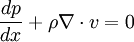
This equation and notation works in much the same way as the temperature equation. This equation describes the motion of water from one place to another at a point without taking into account water that changes form. Inside a given system, the total change in water with time is zero. However, concentrations are allowed to move with the wind.

Pressure thickness:

$\frac{\partial}{\partial t} \frac{\partial p}{\partial \sigma} = u \frac{\partial}{\partial x} x \frac{\partial p}{\partial \sigma} + v \frac{\partial}{\partial y} y \frac{\partial p}{\partial \sigma} + w \frac{\partial}{\partial z} z \frac{\partial p}{\partial \sigma}$

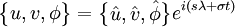
These simplifications make it much easier to understand what is happening in the model. Things like the temperature (potential temperature), precipitable water, and to an extent the pressure thickness simply move from one spot on the grid to another with the wind. The wind is forecasted slightly differently. It uses geopotential, specific heat, the exner function π, and change in sigma coordinate.

Solution to the primitive equations

The analytic solution to the primitive equations involves a sinusoidal oscillation in time and longitude, modulated by coefficients related to height and latitude.

$\begin{Bmatrix}u, v, \phi \end{Bmatrix} = \begin{Bmatrix}\hat u, \hat v, \hat \phi \end{Bmatrix} e^{i(s \lambda + \sigma t)}$

where s and $σ$ are the zonal wavenumber and angular frequency, respectively. The solution represents atmospheric waves and tides.

When the coefficients are separated into their height and latitude components, the height dependence takes the form of propagating or evanescent waves (depending on conditions), while the latitude dependence is given by the Hough functions.

This analytic solution is only possible when the primitive equations are linearized and simplified. Unfortunately many of these simplifications (i.e. no dissipation, isothermal atmosphere) do not correspond to conditions in the actual atmosphere. As a result, a numerical solution which takes these factors into account is often calculated using general circulation models and climate models.

Forecasting temperature

In this form of computer model, the change in temperature at a given location is the easiest thing to forecast. The temperature, given in potential temperature, is simply moved from one spot to another. How?

If temperature changes by 2 degrees every 1 mile north and by 1 degree every 1 mile east:
If you multiply the rate of change in temperature per mile north by the wind speed in the north-south direction in mph, you get the change in temperature per hour contributed from this direction.
If you multiply the rate of change in temperature per mile east by the wind speed in the east-west direction in mph, you get the change in temperature per hour contributed from that direction.
Adding the change given from both directions gives us the total change in temperature per hour. This total change in temperature added to the original temperature will give us our forecast temperature.

Forecasting precipitable water and pressure thickness

The format explained above for calculating the change in temperature is exactly the way the change in precipitable water and pressure thickness can be forecasted. The most difficult calculations involve forecasting the change in wind between run intervals.

References

^ Before 1955: Numerical Models and the Prehistory of AGCMs

Beniston, Martin. From Turbulence to Climate: Numerical Investigations of the Atmosphere with a Hierarchy of Models. Berlin: Springer, 1998.

Firth, Robert. Mesoscale and Microscale Meteorological Model Grid Construction and Accuracy. LSMSA, 2006.

Thompson, Philip. Numerical Weather Analysis and Prediction. New York: The Macmillan Company, 1961.

Pielke, Roger A. Mesoscale Meteorological Modeling. Orlando: Academic Press, Inc., 1984.

U.S. Department of Commerce, National Oceanic and Atmospheric Administration, National Weather Service. National Weather Service Handbook No. 1 - Facsimile Products. Washington, DC: Department of Commerce, 1979.