To use all functions of this page, please activate cookies in your browser.
My watch list
my.chemeurope.com
my.chemeurope.com
With an accout for my.chemeurope.com you can always see everything at a glance – and you can configure your own website and individual newsletter.
- My watch list
- My saved searches
- My saved topics
- My newsletter
Young's modulus
In solid mechanics, Young's modulus (E) is a measure of the stiffness of a given material. It is also known as the Young modulus, modulus of elasticity, elastic modulus or tensile modulus (the bulk modulus and shear modulus are different types of elastic modulus). It is defined as the ratio, for small strains, of the rate of change of stress with strain.[1] This can be experimentally determined from the slope of a stress-strain curve created during tensile tests conducted on a sample of the material. Young's modulus is named after Thomas Young, the 18th Century British scientist. However, the concept was developed in 1727 by Leonhard Euler and the first experiments that used the concept of Young's modulus in its current form were performed by the Italian scientist Giordano Riccati in 1782 - predating Young's work by 25 years[2]. Product highlight
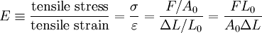
UnitsThe SI unit of modulus of elasticity (E, or less commonly Y) is the pascal. Given the large values typical of many common materials, figures are usually quoted in megapascals or gigapascals. Some use an alternative unit form, kN/mm², which gives the same numeric value as gigapascals. The modulus of elasticity can also be measured in other units of pressure, for example pounds per square inch. UsageThe Young's modulus allows the behavior of a material under load to be calculated. For instance, it can be used to predict the amount a wire will extend under tension, or to predict the load at which a thin column will buckle under compression. Some calculations also require the use of other material properties, such as the shear modulus, density, or Poisson's ratio. Linear vs non-linearFor many materials, Young's modulus is a constant over a range of strains. Such materials are called linear, and are said to obey Hooke's law. Examples of linear materials include steel, carbon fiber, and glass. Rubber and soils (except at very small strains) are non-linear materials. Directional materialsMost metals and ceramics, along with many other materials, are isotropic: their mechanical properties are the same in all directions, but metals and ceramics can be treated to create different grain sizes and orientations. This treatment makes them anisotropic, meaning that Young's modulus will change depending on which direction the force is applied from. However, some materials, particularly those which are composites of two or more ingredients have a "grain" or similar mechanical structure. As a result, these anisotropic materials have different mechanical properties when load is applied in different directions. For example, carbon fiber is much stiffer (higher Young's modulus) when loaded parallel to the fibers (along the grain). Other such materials include wood and reinforced concrete. Engineers can use this directional phenomenon to their advantage in creating various structures in our environment. Copper is an excellent conductor of electricity and is used to transmit electricity over long distance cables, however copper has a relatively low value for Young's modulus at 130 GPa and it tends to stretch in tension. When the copper cable is bound completely in steel wire around its outside this stretching can be prevented as the steel (with a higher value of Young's modulus in tension) takes up the tension that the copper would otherwise experience. CalculationYoung's modulus, E, can be calculated by dividing the tensile stress by the tensile strain: where
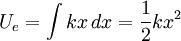
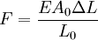
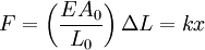
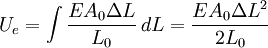
Force exerted by stretched or compressed materialThe Young's modulus of a material can be used to calculate the force it exerts under a specific strain. where F is the force exerted by the material when compressed or stretched by ΔL. From this formula can be derived Hooke's law, which describes the stiffness of an ideal spring: where Elastic potential energyThe elastic potential energy stored is given by the integral of this expression with respect to L: where Ue is the elastic potential energy. The elastic potential energy per unit volume is given by:
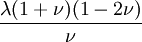
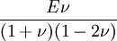
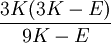
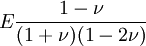
This formula can also be expressed as the integral of Hooke's law: Relation among elastic constantsFor homogeneous isotropic materials simple relations exist between elastic constants (Young's modulus E, shear modulus G, bulk modulus K, and Poisson's ratio ν) that allow calculating them all as long as two are known: Approximate valuesYoung's modulus can vary somewhat due to differences in sample composition and test method. The values here are approximate.
See also
References
|
|||||||||||||||||||||||||||||||||||||||||||||||||||||||||||||||||||||||||||||||||||||||||||||||||||||||||||||||||||||||||||||||||||||||||||||||||||||||||||||||||||||||||||||||||||||||
| This article is licensed under the GNU Free Documentation License. It uses material from the Wikipedia article "Young's_modulus". A list of authors is available in Wikipedia. | |||||||||||||||||||||||||||||||||||||||||||||||||||||||||||||||||||||||||||||||||||||||||||||||||||||||||||||||||||||||||||||||||||||||||||||||||||||||||||||||||||||||||||||||||||||||


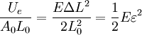 , where
  is the strain in the material.