My watch list

Critical exponent

Critical exponents describe the behaviour of physical quantities near continuous phase transitions. Remarkable about them is that they are universal, i.e. do not depend on details of the physical system, but only on

the dimension of the system,
the range of the interaction,
the spin dimension.

Additional recommended knowledge

Daily Visual Balance Check

What is the Correct Way to Check Repeatability in Balances?

What is the Sensitivity of my Balance?

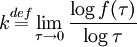
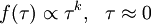
These properties of critical exponents were found in experiments. The experimental results can be theoretically achieved in Mean Field Theory for higher-dimensional systems (4 or more dimensions). The theoretical treatment of lower-dimensional systems (1 or 2 dimensions) is more difficult and requires the Renormalization group.

Definition

Phase transitions occour at a certain temperature, called the critical temperature $T c$ . We want to describe the behaviour of a physical quantity $f$ in terms of a power law around the critical temperature. So we introduce the reduced temperature $τ: = (T - T c) / T c$ , which is zero at the phase transition, and define the critical exponent $k$ .

$k\stackrel{def}{=}\lim_{\tau \to 0}{\log f(\tau) \over \log \tau}$

This results in the power law we were looking for.

$f(\tau) \propto \tau^k,\ \ \tau\approx 0$

The most important critical exponents

Above and below T_c the system has two different phases characterized by an order parameter Ψ, which vanishes at and above T_c.

Let us consider the disordered phase (τ > 0), ordered phase (τ < 0 ) and critical temperature (τ = 0) phases separately. Following the standard convention, the critical exponents related to the ordered phase are primed. We have spontaneous symmetry breaking in the ordered phase. So, we will arbitrarily take any solution in the phase.

Keys
Ψ	order parameter (ρ − ρ_c)/ρ_c for the liquid-gas critical point, magnetization for the Curie point,etc.)
τ	(T − T_c)/T_c
C	specific heat; $-T\frac{\partial^2 F}{\partial T^2}$
J	source field (e.g. (P − P_c)/P_c where P is the pressure and P_c the critical pressure for the liquid-gas critical point, the magnetic field H for the Curie point )
χ	the susceptibility/compressibility/etc.; $\frac{\partial \Psi}{\partial J}$
ξ	correlation length
d	the number of spatial dimensions
$\left\langle \psi(\vec{x}) \psi(\vec{y}) \right\rangle$	the correlation function

The following entries are evaluated at J = 0 (except for the δ entry)

Critical exponents for τ > 0 (disordered phase)
Greek letter	relation
α	C ~ τ^−α
γ	χ ~ τ^−γ
ν	ξ ~ τ^−ν

Critical exponents for τ < 0 (ordered phase)
Greek letter	relation
α'	C ~ (−τ)^−α'
β	Ψ ~ (−τ)^β
γ'	χ ~ (−τ)^−γ'
ν'	ξ ~ (−τ)^−ν'

Critical exponents for τ = 0
δ	J ~ ψ^δ
η	$\left\langle \psi(0) \psi(r) \right\rangle \sim r^{-d+2-\eta}$

These relations are accurate close to the critical point in two- and three-dimensional systems. In four dimensions, however, the power laws are modified by logarithmic factors. This problem does not appear in 3.99 dimensions, though.

α = α'

γ = γ'

ν = ν'

The classical (Landau theory aka mean field theory) values are

α = α' = 0

β = 1/2

γ = γ' = 1

δ = 3

If we add derivative terms turning it into a mean field Landau-Ginzburg theory, we get

η = 0

ν = 1 / 2

The most accurately measured value of $α$ is −0.0127 for the phase transition of superfluid helium (the so-called lambda-transition). The value was measured in a satellite to minimize pressure differences in the sample (see here). This result agrees with theoretical prediction obtained by variational perturbation theory (see here or here).

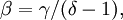
Critical exponents are denoted by Greek letters. They fall into universality classes and obey scaling relations such as

$\beta=\gamma/(\delta-1),\,$

$\nu=\gamma/(2-\eta).\,$

The critical exponents can be computed from conformal field theory.

Critical exponent

Additional recommended knowledge

Daily Visual Balance Check

What is the Correct Way to Check Repeatability in Balances?

What is the Sensitivity of my Balance?

Definition

The most important critical exponents

See also

About chemeurope.com

About LUMITOS

Advertise with LUMITOS