My watch list

Home
Encyclopedia
Accidental_release_source_terms

Accidental release source terms

Accidental release source terms are the mathematical equations that quantify the flow rate at which accidental releases of air pollutants into the ambient environment can occur at industrial facilities such as petroleum refineries, petrochemical plants, natural gas processing plants, oil and gas transportation pipelines, chemical plants, and many other industrial activities. Governmental regulations in a good many countries require that the probability of such accidental releases be analyzed and their quantitative impact upon the environment and human health be determined so that mitigating steps can be planned and implemented.

There are a number of mathematical calculation methods for determining the flow rate at which gaseous and liquid pollutants might be released from various types of accidents. Such calculational methods are referred to as source terms, and this article on accidental release source terms explains some of the calculation methods used for determining the mass flow rate at which gaseous pollutants may be accidentally released.

Additional recommended knowledge

Guide to balance cleaning: 8 simple steps

Weighing the right way

Correct Test Weight Handling Guide: 12 Practical Tips

1 Accidental release of pressurized gas
- 1.1 Ramskill's equation for non-choked mass flow
2 Evaporation of non-boiling liquid pool
3 Evaporation of boiling cold liquid pool
4 Adiabatic flash of liquified gas release
5 See also
6 References

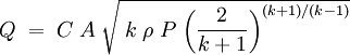
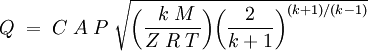
Accidental release of pressurized gas

When gas stored under pressure in a closed vessel is discharged to the atmosphere through a hole or other opening, the gas velocity through that opening may be choked (i.e., it has attained a maximum) or it may be non-choked.

Choked velocity, also referred to as sonic velocity, occurs when the ratio of the absolute source pressure to the absolute downstream pressure is equal to or greater than [(k + 1) ÷ 2 ]^{k÷(k - 1 )}, where k is the specific heat ratio of the discharged gas (sometimes called the isentropic expansion factor and sometimes denoted as $γ$ ).

For many gases, k ranges from about 1.09 to about 1.41, and therefore [(k + 1) ÷ 2 ]^{k÷(k - 1 )} ranges from 1.7 to about 1.9, which means that choked velocity usually occurs when the absolute source vessel pressure is at least 1.7 to 1.9 times as high as the absolute downstream ambient atmospheric pressure.

When the gas velocity is choked, the equation for the mass flow rate in SI metric units is:^[1]^[2]^[3]^[4]

$Q\;=\;C\;A\;\sqrt{\;k\;\rho\;P\;\bigg(\frac{2}{k+1}\bigg)^{(k+1)/(k-1)}}$

or this equivalent form:

$Q\;=\;C\;A\;P\;\sqrt{\bigg(\frac{\;\,k\;M}{Z\;R\;T}\bigg)\bigg(\frac{2}{k+1}\bigg)^{(k+1)/(k-1)}}$

For the above equations, it is important to note that although the gas velocity reaches a maximum and becomes choked, the mass flow rate is not choked. The mass flow rate can still be increased if the source pressure is increased.

Whenever the ratio of the absolute source pressure to the absolute downstream ambient pressure is less than [ ( k + 1 ) ÷ 2 ]^{k ÷ ( k - 1 )}, then the gas velocity is non-choked (i.e., sub-sonic) and the equation for mass flow rate is:

$Q\;=\;C\;A\;\sqrt{\;2\;\rho\;P\;\bigg(\frac{k}{k-1}\bigg)\Bigg[\,\bigg(\frac{\;P_A}{P}\bigg)^{2/k}-\;\,\bigg(\frac{\;P_A}{P}\bigg)^{(k+1)/k}\;\Bigg]}$

or this equivalent form:

$Q\;=\;C\;A\;P\;\sqrt{\bigg(\frac{2\;M}{Z\;R\;T}\bigg)\bigg(\frac{k}{k-1}\bigg)\Bigg[\,\bigg(\frac{\;P_A}{P}\bigg)^{2/k}-\;\,\bigg(\frac{\;P_A}{P}\bigg)^{(k+1)/k}\;\Bigg]}$

where:
Q	= mass flow rate, kg/s
C	= discharge coefficient, dimensionless (usually about 0.72)
A	= discharge hole area, m²
k	= c_p/c_v of the gas
c_p	= specific heat of the gas at constant pressure
c_v	= specific heat of the gas at constant volume
$ρ$	= real gas density at P and T, kg/m³
P	= absolute upstream pressure, Pa
P_A	= absolute ambient or downstream pressure, Pa
M	= the gas molecular mass, kg/kmole (also known as the molecular weight)
R	= the Universal Gas Law Constant = 8314.5 Pa·m³/(kmole·K)
T	= absolute upstream gas temperature, K
Z	= the gas compressibility factor at P and T, dimensionless

The above equations calculate the initial instantaneous mass flow rate for the pressure and temperature existing in the source vessel when a release first occurs. The initial instantaneous flow rate from a leak in a pressurized gas system or vessel is much higher than the average flow rate during the overall release period because the pressure and flow rate decrease with time as the system or vessel empties. Calculating the flow rate versus time since the initiation of the leak is much more complicated, but more accurate. Two equivalent methods for performing such calculations are presented and compared at www.air-dispersion.com/feature2.html.

The technical literature can be very confusing because many authors fail to explain whether they are using the universal gas law constant R which applies to any ideal gas or whether they are using the gas law constant R_s which only applies to a specific individual gas. The relationship between the two constants is R_s = R/M.

Notes:

The above equations are for a real gas.
For an ideal gas, Z = 1 and ρ is the ideal gas density.
kmole = 1000 moles = 1000 gram-moles = kilogram-mole.

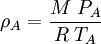
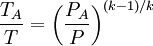
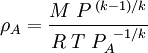
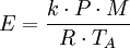
Ramskill's equation for non-choked mass flow

P.K. Ramskill's equation ^[5]^[6] for the non-choked flow of an ideal gas is shown below as equation (1):

(1) $Q = C \;\rho_A\;A\;\sqrt{\frac{\;\,2\;P}{\rho}\cdot\frac{k}{k-1}\cdot{\Bigg[\; 1 - {\bigg(\frac{P_A}{P}\bigg)^{(k-1)/k)}}\Bigg]}}$

The gas density, $ρ$ _A, in Ramskill's equation is the ideal gas density at the downstream conditions of temperature and pressure and it is defined in equation (2) using the ideal gas law:

(2) $\rho_A = \frac{M\;P_A}{R \;T_A}$

Since the downstream temperature T_A is not known, the isentropic expansion equation below ^[7] is used to determine T_A in terms of the known upstream temperature T:

(3) $\frac{T_A}{T} = \bigg(\frac{P_A}{P}\bigg)^{(k-1)/k}$

Combining equations (2) and (3) results in equation (4) which defines $ρ$ _A in terms of the known upstream temperature T:

(4) $\rho_A = \frac{M \;P^{\;(k-1)/k}}{R \;T \;P_A^{\ -1/k}}$

Using equation (4) with Ramskill's equation (1) to determine non-choked mass flow rates for ideal gases gives identical results to the results obtained using the non-choked flow equation presented in the previous section above.

Evaporation of non-boiling liquid pool

Three different methods of calculating the rate of evaporation from a non-boiling liquid pool are presented in this section. The results obtained by the three methods are somewhat different.

The U.S. Air Force method

$E=(4.161\times{10^{-5}})\cdot u^{0.75}\cdot T_F\cdot M\cdot (P_S / P_H)$

where:
E	= evaporation flux, (kg/min)/m² of pool surface
u	= windspeed just above the liquid surface, m/s
T_A	= absolute ambient temperature, K
T_F	= pool liquid temperature correction factor, dimensionless
T_P	= pool liquid temperature, °C
M	= pool liquid molecular weight, dimensionless
P_S	= pool liquid vapor pressure at ambient temperature, mmHg
P_H	= hydrazine vapor pressure at ambient temperature, mmHg (see equation below)

If T_P = 0 °C or less, then T_F = 1.0
If T_P > 0 °C, then T_F = 1.0 + 0.0043 T_P²

$P_H = 760\cdot e^{65.3319-(7245.2/T_A)-(8.22\;ln\;T_a) + (0.0061557\;T_A)}$

where:
$e$	= 2.7183, the base of the natural logarithm system
$l n$	= natural logarithm

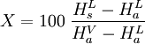
The U.S. EPA method

The following equations are for predicting the rate at which liquid evaporates from the surface of a pool of liquid which is at or near the ambient temperature. The equations were developed by the United States Environmental Protection Agency using units which were a mixture of metric usage and United States usage.^[3] The non-metric units have been converted to metric units for this presentation.

$E = \frac{0.1268\cdot A\cdot P\cdot M^{0.667}\cdot u^{0.78}}{T}$

where:
E	= evaporation rate, kg/min
u	= windspeed just above the pool liquid surface, m/s
M	= pool liquid molecular weight, dimensionless
A	= surface area of the pool liquid, m²
P	= vapor pressure of the pool liquid at the pool temperature, kPa
T	= pool liquid absolute temperature, K

The U.S. EPA also defined the pool depth as 0.01 m (i.e., 1 cm) so that the surface area of the pool liquid could be calculated as:

A = ( pool volume, in m³ ) / (0.01)

Notes:

1 kPa = 0.0102 kgf/cm² = 0.01 bar
mol = mole
atm = atmosphere

Stiver and Mackay's method

The following equations are for predicting the rate at which liquid evaporates from the surface of a pool of liquid which is at or near the ambient temperature. The equations were developed by Warren Stiver and Dennis Mackay of the Chemical Engineering Department at the University of Toronto. ^[8]

$E = \frac{k\cdot P\cdot M}{R\cdot T_A}$

where:
E	= evaporation flux, (kg/s)/m² of pool surface
k	= mass transfer coefficient, m/s = 0.002 u
T_A	= absolute ambient temperature, K
M	= pool liquid molecular weight, dimensionless
P	= pool liquid vapor pressure at ambient temperature, Pa
R	= the universal gas law constant = 8314.5 Pa·m³/(kmol·K)
u	= windspeed just above the liquid surface, m/s

Evaporation of boiling cold liquid pool

The following equation is for predicting the rate at which liquid evaporates from the surface of a pool of cold liquid (i.e., at a liquid temperature of about 0 °C or less). ^[2]

$E = ( 0.0001\;M) (7.7026-0.0288\;B)\;e^{-(0.0077\;B)-0.1376}$

where:
E	= evaporation flux, (kg/min)/m² of pool surface
B	= pool liquid atmospheric boiling point, °C
M	= pool liquid molecular weight, dimensionless
e	= the base of the natural logarithm system = 2.7183

Adiabatic flash of liquified gas release

Liquified gases such as ammonia or chlorine are often stored in cylinders or vessels at ambient temperatures and pressures well above atmospheric pressure. When such a liquified gas is released into the ambient atmosphere, the resultant reduction of pressure causes some of the liquified gas to vaporize immediately. This is known as "adiabatic flashing" and the following equation, derived from a simple heat balance, is used to predict how much of the liquified gas is vaporized.

$X = 100\;\frac{H_s^L - H_a^L}{H_a^V - H_a^L}$

where:
X	= weight percent vaporized
H_s^L	= source liquid enthalpy at source temperature and pressure, J/kg
H_a^V	= flashed vapor enthalpy at atmospheric boiling point and pressure, J/kg
H_a^L	= residual liquid enthalpy at atmospheric boiling point and pressure, J/kg

If the enthalpy data required for the above equation is unavailable, then the following equation may be used.

$X = 100\cdot c_p\cdot (T_s - T_b)/H$

where:
X	= weight percent vaporized
c_p	= source liquid specific heat, J/(kg °C)
T_s	= source liquid absolute temperature, K
T_b	= source liquid absolute atmospheric boiling point, K
H	= source liquid heat of vaporization at atmospheric boiling point, J/kg

References

^ Perry's Chemical Engineers' Handbook, Sixth Edition, McGraw-Hill Co., 1984.
^ ^a ^b ^c Handbook of Chemical Hazard Analysis Procedures, Appendix B, Federal Emergency Management Agency, U.S. Dept. of Transportation, and U.S. Environmental Protection Agency, 1989. Also provides the references below:
– Clewell, H.J., A Simple Method For Estimating the Source Strength Of Spills Of Toxic Liquids, Energy Systems Laboratory, ESL-TR-83-03, 1983.
– Ille, G. and Springer, C., The Evaporation And Dispersion Of Hydrazine Propellants From Ground Spill, Environmental Engineering Development Office, CEEDO 712-78-30, 1978.
– Kahler, J.P., Curry, R.C. and Kandler, R.A.,Calculating Toxic Corridors Air Force Weather Service, AWS TR-80/003, 1980.
Handbook of Chemical Hazard Analysis, Appendix B Click on PDF icon, wait and then scroll down to page 391 of 520 PDF pages.
^ ^a ^b "Risk Management Program Guidance For Offsite Consequence Analysis", U.S. EPA publication EPA-550-B-99-009, April 1999. Guidance for Offsite Consequence Analysis
^ "Methods For The Calculation Of Physical Effects Due To Releases Of Hazardous Substances (Liquids and Gases)", PGS2 CPR 14E, Chapter 2, The Netherlands Organization Of Applied Scientific Research, The Hague, 2005. PGS2 CPR 14E
^ CACHE Newsletter No.48, Spring 1999 Gierer, C. and Hyatt, N.,Using Source Term Analysis Software for Calculating Fluid Flow Release Rates Dyadem International Ltd.
^ Ramskill, P.K. (1986), Discharge Rate Calculation Methods for Use In Plant Safety Assessments, Safety and Reliability Directory, United Kingdom Atomic Energy Authority
^ Isentropic Compression or Expansion
^ Stiver, W. and Mackay, D., A Spill Hazard Ranking System For Chemicals, Environment Canada First Technical Spills Seminar, Toronto, Canada, 1993.

Category: Chemical engineering

This article is licensed under the GNU Free Documentation License. It uses material from the Wikipedia article "Accidental_release_source_terms". A list of authors is available in Wikipedia.