To use all functions of this page, please activate cookies in your browser.
My watch list
my.chemeurope.com
my.chemeurope.com
With an accout for my.chemeurope.com you can always see everything at a glance – and you can configure your own website and individual newsletter.
- My watch list
- My saved searches
- My saved topics
- My newsletter
Euler-Bernoulli beam equation
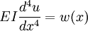
Euler-Bernoulli beam theory or just beam theory is a simplification of the linear isotropic theory of elasticity which provides a means of calculating the load-carrying and deflection characteristics of beams. It was first enunciated circa 1750, but was not applied on a large scale until the development of the Eiffel Tower and the Ferris Wheel in the late 19th century. Following these successful demonstrations, it quickly became a cornerstone of engineering and an enabler of the Second Industrial Revolution. Additional analysis tools have been developed such as plate theory and finite element analysis, but the simplicity of beam theory makes it an important tool in the sciences, especially structural and mechanical engineering. Product highlight
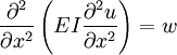
HistoryThe prevailing consensus is that Galileo Galilei made the first attempts at developing a theory of beams, but recent studies argue that Leonardo da Vinci was the first to make the crucial observations. Da Vinci lacked Hooke's law and calculus to complete the theory, whereas Galileo was held back by an incorrect assumption he made.[1] The Bernoulli beam is named after Jacob Bernoulli, who made the significant discoveries. Leonhard Euler and Daniel Bernoulli were the first to put together a useful theory circa 1750.[2] At the time, science and industrial art were generally seen as very distinct fields, and there was considerable doubt that a mathematical product of academia could be trusted for practical safety applications. Bridges and buildings continued to be designed by precedent until the late 19th century, when the Eiffel Tower and Ferris wheel demonstrated the validity of the theory on large scales. The beam equationThe Euler-Bernoulli Beam Equation is based on 5 assumptions about a bending beam. Colloquially stated, they are that (1) calculus is valid and is applicable to bending beams More rigorously stated, these assumptions are: (1) continuum mechanics is valid for a bending beam With these assumptions, we can derive the following equation governing the relationship between the beam's deflection and the applied load. This is the Euler-Bernoulli equation. The curve u(x) describes the deflection u of the beam at some position x (recall that the beam is modeled as a one dimensional object). w is a distributed load, in other words a force per unit length (analogous to pressure being a force per area); it may be a function of x, u, or other variables. Note that E is the elastic modulus and that I is the second moment of area. I must be calculated with respect to the centroidal axis perpendicular to the applied loading, for an Euler-Bernoulli beam not under any axial loading this axis is called the neutral axis. Often, u = u(x), w = w(x), and EI is a constant, so that: This equation is very common in engineering practice: it describes the deflection of a uniform, static beam. Successive derivatives of u have important meaning:
StressBesides deflection, the beam equation describes forces and moments and can thus be used to describe stresses. For this reason, the Euler-Bernoulli beam equation is widely used in engineering, especially civil and mechanical, to determine the strength (as well as deflection) of beams under bending. Both the bending moment and the shear force cause stresses in the beam. The stress due to shear force is maximum along the neutral axis of the beam, and the maximum tensile stress is at either the top or bottom surfaces. Thus the maximum principal stress in the beam may be neither at the surface nor at the center but in some general area. However, shear force stresses are negligible in comparison to bending moment stresses in all but the stockiest of beams as well as the fact that stress concentrations commonly occur at surfaces, meaning that the maximum stress in a beam is likely to be at the surface. It can be shown that the tensile stress experienced by the beam may be expressed as: Here, c is a position along u, it is the distance from the neutral axis to a point of interest; M is the bending moment. Note that this equation implies that "pure" bending (of positive sign) will cause zero stress at the neutral axis, positive (tensile) stress at the "top" of the beam, and negative (compressive) stress at the bottom of the beam; this also implies that the maximum stress will be at the top surface and the minimum at the bottom. This bending stress may be superimposed with axially applied stresses, which will cause a shift in the neutral (zero stress) axis. Boundary considerationsThe beam equation contains a fourth order derivative in x, hence it mandates at most four conditions, normally boundary conditions. The boundary conditions usually model supports, they can also model point loads, moments, or other effects.
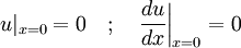
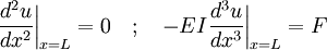
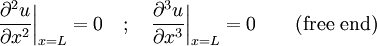
An example is a cantilever beam: a beam that is completely fixed at one end and completely free at the other. "Completely fixed" means that at the left end both deflection and slope are zero; "completely free" implies (though it may or may not be obvious) that at the right end both shear force and bending moment are zero. Taking the x coordinate of the left end as 0 and the right end as L (the length of the beam), these statements translate to the following set of boundary conditions (assume EI is a constant): Some commonly encountered boundary conditions include:
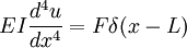
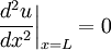
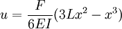
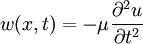
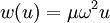
Loading considerationsApplied loading may be represented either through boundary conditions or through the distributed function w. Using distributed loading is often favorable for simplicity. Boundary conditions are, however, often used to model loads depending on context, the practice is especially common in vibration analysis. By nature, the distributed load is very often represented in a piecewise manner, since in practice a load isn't typically a "nice" continuous function. Point loads can be modeled with help of the dirac delta function. For example, consider a static uniform cantilever beam of length L with an upward point load F applied at the free end. Using boundary conditions, this may be modeled through: Using the Dirac function, Note that shear force boundary condition (third derivative) is removed, otherwise there would be a contradiction. These are equivalent boundary value problems, and both yield the following solution: The application of several point loads at different locations will lead to u(x) being a piecewise function. Use of the Dirac function greatly simplifies such situations; otherwise the beam would have to be divided into sections, each with four boundary conditions solved separately. A well organized family of functions called Singularity functions are often used as a shorthand for the Dirac function, its derivative, and its antiderivatives. Clever formulation of the load distribution allows for many interesting phenomena to be modeled. As an example, the vibration of a beam can be accounted for using the load function: Where μ is the linear density of the beam, not necessarily a constant. With this time-dependent loading, the beam equation will be a partial differential equation. Another interesting example describes the deflection of a beam rotating with a constant angular velocity of ω: This is a centripetal force distribution. Note that in this case, w is a function of the displacement (the dependent variable), and the beam equation will be an autonomous ordinary differential equation. ExtensionsThe kinematic assumptions upon which the Euler-Bernoulli beam theory is founded allow it to be extended to more advanced analysis. Simple superposition allows for three dimensional transverse loading. Using alternative constitutive equations can allow for viscoelastic or plastic beam deformation. Euler-Bernoulli beam theory can also be extended to the analysis of curved beams, beam buckling, composite beams, and geometrically nonlinear beam deflection. Euler-Bernoulli beam theory does not account for the effects of transverse shear strain. As a result the Euler-Bernoulli beam theory underpredicts deflections and overpredicts natural frequencies. For thin beams (beam length to thickness ratios of the order 20 or more) these effects are of minor importance. For thick beams, however, these effects can be significant. More advanced beam theories such as the Timoshenko beam theory (developed by the Russian-born scientist Stephen Timoshenko) have been developed to account for these effects. See alsoReferences
|
|
| This article is licensed under the GNU Free Documentation License. It uses material from the Wikipedia article "Euler-Bernoulli_beam_equation". A list of authors is available in Wikipedia. |


 is the deflection.
 is the slope of the beam.
 is the
 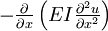 is the
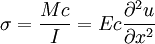
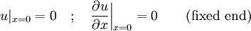
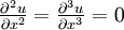
 represents a fixed support.
 represents a pin connection (deflection and moment fixed to zero).
 represents no connection (no restraint) and no load.
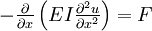 represents the application of a point load F.