To use all functions of this page, please activate cookies in your browser.
My watch list
my.chemeurope.com
my.chemeurope.com
With an accout for my.chemeurope.com you can always see everything at a glance – and you can configure your own website and individual newsletter.
- My watch list
- My saved searches
- My saved topics
- My newsletter
Maxwell–Boltzmann statistics
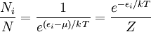
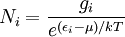
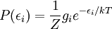
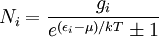
In statistical mechanics, Maxwell–Boltzmann statistics describes the statistical distribution of material particles over various energy states in thermal equilibrium, when the temperature is high enough and density is low enough to render quantum effects negligible. Maxwell–Boltzmann statistics are therefore applicable to almost any terrestrial phenomena for which the temperature is above a few tens of kelvins. The expected number of particles with energy εi for Maxwell–Boltzmann statistics is Ni where: where:
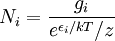
Equivalently, the distribution is sometimes expressed as where the index i now specifies a particle's state rather than the set of all states with energy εi Fermi-Dirac and Bose-Einstein statistics apply when quantum effects have to be taken into account and the particles are considered "indistinguishable". The quantum effects appear if the concentration of particles (N/V) ≥ nq (where nq is the quantum concentration). The quantum concentration is when the interparticle distance is equal to the thermal de Broglie wavelength i.e. when the wavefunctions of the particles are touching but not overlapping. As the quantum concentration depends on temperature; high temperatures will put most systems in the classical limit unless they have a very high density e.g. a White dwarf. Fermi-Dirac statistics apply to fermions (particles that obey the Pauli exclusion principle), Bose-Einstein statistics apply to bosons. Both Fermi-Dirac and Bose-Einstein become Maxwell-Boltzmann statistics at high temperatures or low concentrations. Maxwell-Boltzmann statistics are often described as the statistics of "distinguishable" classical particles. In other words the configuration of particle A in state 1 and particle B in state 2 is different from the case where particle B is in state 1 and particle A is in state 2. When this idea is carried out fully, it yields the proper (Boltzmann) distribution of particles in the energy states, but yields non-physical results for the entropy, as embodied in Gibbs paradox. These problems disappear when it is realized that all particles are in fact indistinguishable. Both of these distributions approach the Maxwell-Boltzmann distribution in the limit of high temperature and low density, without the need for any ad hoc assumptions. Maxwell-Boltzmann statistics are particularly useful for studying gases. Fermi-Dirac statistics are most often used for the study of electrons in solids. As such, they form the basis of semiconductor device theory and electronics. Product highlight
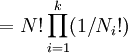
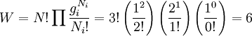
A derivation of the Maxwell–Boltzmann distributionIn this particular derivation, the Boltzmann distribution will be derived using the assumption of distinguishable particles, even though the ad hoc correction for Boltzmann counting is ignored, the results remain valid. Suppose we have a number of energy levels, labelled by index i , each level having energy εi and containing a total of Ni particles. To begin with, let's ignore the degeneracy problem. Assume that there is only one way to put Ni particles into energy level i. The number of different ways of performing an ordered selection of one object from N objects is obviously N. The number of different ways of selecting 2 objects from N objects, in a particular order, is thus N(N − 1) and that of selecting n objects in a particular order is seen to be N! / (N − n)!. The number of ways of selecting 2 objects from N objects without regard to order is N(N − 1) divided by the number of ways 2 objects can be ordered, which is 2!. It can be seen that the number of ways of selecting n objects from N objects without regard to order is the binomial coefficient: N! / n!(N − n)!. If we have a set of boxes numbered where the extended product is over all boxes containing one or more objects. If the i-th box has a "degeneracy" of gi, that is, it has gi sub-boxes, such that any way of filling the i-th box where the number in the sub-boxes is changed is a distinct way of filling the box, then the number of ways of filling the i-th box must be increased by the number of ways of distributing the Ni objects in the gi boxes. The number of ways of placing Ni distinguishable objects in gi boxes is For example, suppose we have three particles, a, b, and c, and we have three energy levels with degeneracies 1, 2, and 1 respectively. There are 6 ways to arrange the 3 particles so that N1 = 2, N2 = 1 and N3 = 0.
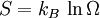
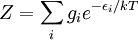
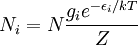
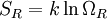
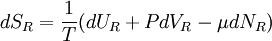
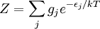
The six ways are calculated from the formula: We wish to find the set of Ni for which W is maximized, subject to the constraint that there be a fixed number of particles, and a fixed energy. The maxima of W and ln(W) are achieved by the same values of Ni and, since it is easier to accomplish mathematically, we will maximise the latter function instead. We constrain our solution using Lagrange multipliers forming the function: Using Stirling's approximation for the factorials and taking the derivative with respect to Ni, and setting the result to zero and solving for Ni yields the Maxwell–Boltzmann population numbers: It can be shown thermodynamically that β = 1/kT where k is Boltzmann's constant and T is the temperature, and that α = -μ/kT where μ is the chemical potential, so that finally: Note that the above formula is sometimes written: where z = exp(μ / kT) is the absolute activity. Alternatively, we may use the fact that to obtain the population numbers as where Z is the partition function defined by: Another derivationIn the above discussion, the Boltzmann distribution function was obtained via directly analysing the multiplicities of a system. Alternatively, one can make use of the canonical ensemble. In a canonical ensemble, a system is in thermal contact with a reservoir. While energy is free to flow between the system and the reservoir, the reservoir is thought to have infinitely large heat capacity as to maintain constant temperature, T, for the combined system. In the present context, our system is assumed to be have energy levels εi with degeneracies gi. As before, we would like to calculate the probability that our system has energy εi. If our system is in state Since the entropy of the reservoir Next we recall the thermodynamic identity:
In a canonical ensemble, there is no exchange of particles, so the dNR term is zero. Similarly, dVR = 0. This gives
where
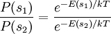
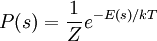
which implies, for any state s of the system
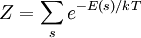
where Z is an appropriately chosen "constant" to make total probability 1. (Z is constant provided that the temperature T is invariant.) It is obvious that
where the index s runs through all microstates of the system.[1] If we index the summation via the energy eigenvalues instead of all possible states, degeneracy must be taken into account. The probability of our system having energy εi is simply the sum of the probabilities of all corresponding microstates: where, with obvious modification,
this is the same result as before. Comments
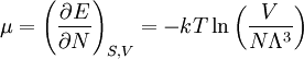
Limits of applicabilityThe Bose–Einstein and Fermi–Dirac distributions may be written: Assuming the minimum value of εi is small, it can be seen that the condition under which the Maxwell–Boltzmann distribution is valid is when For an ideal gas, we can calculate the chemical potential using the development in the Sackur–Tetrode article to show that: where E is the total internal energy, S is the entropy, V is the volume, and Λ is the thermal de Broglie wavelength. The condition for the applicability of the Maxwell–Boltzmann distribution for an ideal gas is again shown to be
References
Carter, Ashley H., "Classical and Statistical Thermodynamics", Prentice-Hall, Inc., 2001, New Jersey. See alsoCategories: Statistical mechanics | Particle statistics |
||||||||||||||||||||||||||||||||||||||||||||||||||||||
| This article is licensed under the GNU Free Documentation License. It uses material from the Wikipedia article "Maxwell–Boltzmann_statistics". A list of authors is available in Wikipedia. | ||||||||||||||||||||||||||||||||||||||||||||||||||||||


 , the number of ways of selecting
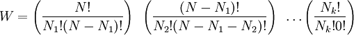
 . Thus the number of ways (
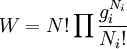


 , then there would be a corresponding number of microstates available to the reservoir. Call this number
  . By assumption, the combined system (of the system we are interested in and the reservoir) is isolated, so all microstates are equally probable. Therefore, for instance, if
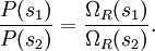
 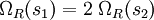 , we can conclude that our system is twice as likely to be in state
  . In general, if
  is the probability that our system is in state
  ,
,
 , the above becomes
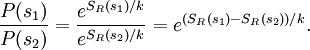
 .
.
 ,
,
 and
and  denote the energies of the reservoir and the system at
  :
:
 ,
,
 ,
,
 ,
,
 ,
,


Last viewed


