My watch list

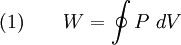
Thermodynamic cycle

A thermodynamic cycle is a series of thermodynamic processes which returns a system to its initial state. Properties depend only on the thermodynamic state and thus do not change over a cycle. Variables such as heat and work are not zero over a cycle, but rather are process dependent. The first law of thermodynamics dictates that the net heat input is equal to the net work output over any cycle. The repeating nature of the process path allows for continuous operation, making the cycle an important concept in thermodynamics. Thermodynamic cycles often use quasistatic processes to model the workings of actual devices.

A thermodynamic cycle is a closed loop on a P-V diagram. A P-V diagrams X axis shows volume (V) and Y axis shows pressure (P). The area enclosed by the loop is the work (W) done by the process:

$\text{(1)} \qquad W = \oint P \ dV$ .

This work is equal to the balance of heat (Q) transferred into the system:

$\text{(2)} \qquad W = Q = Q_{in} - Q_{out}$ .

Equation (2) makes a cyclic process similar to an isothermal process: even though the internal energy changes during the course of the cyclic process, when the cyclic process finishes the system's energy is the same as the energy it had when the process began.

If the cyclic process moves clockwise around the loop, then it represents a heat engine, and W will be positive. If it moves counterclockwise then it represents a heat pump, and W will be negative.

Additional recommended knowledge

Guide to balance cleaning: 8 simple steps

How to quickly check pipettes?

What is the Sensitivity of my Balance?

1 Classes
- 1.1 Thermodynamic power cycles
- 1.2 Thermodynamic heat pump and refrigeration cycle
2 Types of thermodynamic cycles
3 State Functions and Entropy
- 3.1 Demonstration
  - 3.1.1 Part 1
  - 3.1.2 Part 2
- 3.2 Conclusion
4 References
5 See also

Classes

Two primary classes of thermodynamic cycles are power cycles and heat pump cycles. Power cycles are cycles which convert some heat input into a mechanical work output, while heat pump cycles transfer heat from low to high temperatures using mechanical work input. Cycles composed entirely of quasistatic processes can operate as power or heat pump cycles by controlling the process direction. On a pressure-volume or Temperature-entropy diagram, the clockwise and counterclockwise directions indicate power and heat pump cycles, respectively.

Thermodynamic power cycles

Main article: Heat engine

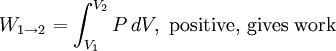
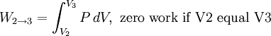
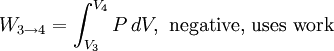
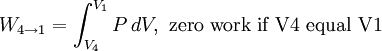
Thermodynamic power cycles are the basis for the operation of heat engines, which supply most of the world's electric power and run almost all motor vehicles. Power cycles can be divided according to the type of heat engine they seek to model. The most common cycles that model internal combustion engines are the Otto cycle, which models gasoline engines and the Diesel cycle, which models diesel engines. Cycles that model external combustion engines include the Brayton cycle, which models gas turbines, and the Rankine cycle, which models steam turbines.

For example the pressure-volume mechanical work done in the heat engine cycle, consisting of 4 thermodynamic processes, is:

$\text{(3)} \qquad W = W_{1\to 2} + W_{2\to 3} + W_{3\to 4} + W_{4\to 1}$

$W_{1\to 2} = \int_{V_1}^{V_2} P \, dV, \, \, \text{positive, gives work}$

$W_{2\to 3} = \int_{V_2}^{V_3} P \, dV, \, \, \text{zero work if V2 equal V3}$

$W_{3\to 4} = \int_{V_3}^{V_4} P \, dV, \, \, \text{negative, uses work}$

$W_{4\to 1} = \int_{V_4}^{V_1} P \, dV, \, \, \text{zero work if V4 equal V1}$

If no volume change happens in process 4->1 and 2->3, equation (3) simplifies to:

$\text{(4)} \qquad W = W_{1\to 2} + W_{3\to 4}$

Thermodynamic heat pump and refrigeration cycle

Main article: Heat pump and refrigeration cycle

Thermodynamic heat pump and refrigeration cycles are the models for heat pumps and refrigerators. The difference between the two is that heat pumps are intended to keep a place warm and refrigerators designed to cool it. The most common refrigeration cycle is the vapor compression cycle, which models systems using refrigerants that change phase. The absorption refrigeration cycle is an alternative that absorbs the refrigerant in a liquid solution rather than evaporating it. Gas refrigeration cycles include the reversed Brayton cycle and the Linde-Hampson cycle. Regeneration in gas refrigeration allows for the liquefaction of gases.

Types of thermodynamic cycles

A thermodynamic cycle can (ideally) be made out of 3 or more thermodynamic processes (typical 4). The processes can be any of these:

isothermal process (at constant temperature, maintained with heat added or removed from a heat source or sink)
isobaric process (at constant pressure)
isometric / isochoric process (at constant volume)
adiabatic process (no heat is added or removed from the working fluid)
- isentropic process, reversible adiabatic process (no heat is added or removed from the working fluid - and the entropy is constant)
isenthalpic process (the enthalpy is constant)

Some examples are as follows:


Cycle\Process	Compression	Heat Addition	Expansion	Heat Rejection
Power cycles normally with external combustion - or heat pump cycles
Ericsson (First, 1833) Brayton	adiabatic	isobaric	adiabatic	isobaric
Bell Coleman (Reverse Brayton)	adiabatic	isobaric	adiabatic	isobaric
Carnot	isentropic	isothermal	isentropic	isothermal
Stoddard	adiabatic	isometric	adiabatic	isometric
Stirling	isothermal	isometric	isothermal	isometric
Ericsson (Second, 1853)	isothermal	isobaric	isothermal	isobaric
Power cycles normally with internal combustion
Otto (Petrol)	adiabatic	isometric	adiabatic	isometric
Diesel	adiabatic	isobaric	adiabatic	isometric
Brayton (Jet)	adiabatic	isobaric	adiabatic	isobaric
Lenoir (pulse jet) (Note: 3 of the 4 processes are different)	isobaric	isometric	adiabatic	isobaric

Carnot cycle

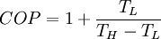
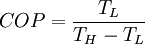
Main article: Carnot cycle

The Carnot cycle is a cycle composed of the totally reversible processes of isentropic compression and expansion and isothermal heat addition and rejection. The thermal efficiency of a Carnot cycle depends only on the temperatures in Kelvin of the two reservoirs in which heat transfer takes place, and for a power cycle is:

$\eta=1-\frac{T_L}{T_H}$

where $T L$ is the lowest cycle temperature and $T H$ the highest. For Carnot refrigeration cycles the coefficient of performance for a heat pump is:

$\ COP = 1+\frac{T_L}{T_H - T_L}$

and for a refrigerator the coefficient of performance is:

$\ COP = \frac{T_L}{T_H - T_L}$

The second law of thermodynamics limits the efficiency and COP for all cyclic devices to levels at or below the Carnot efficiency. The Stirling cycle and Ericsson cycle are two other reversible cycles that use regeneration to obtain isothermal heat transfer.

Ideal cycle

An ideal cycle is constructed out of:

TOP and BOTTOM of the loop: a pair of parallel isobaric processes
LEFT and RIGHT of the loop: a pair of parallel isochoric processes

Otto cycle

Main article: Otto cycle

An Otto cycle is constructed out of:

TOP and BOTTOM of the loop: a pair of quasi-parallel adiabatic processes
LEFT and RIGHT sides of the loop: a pair of parallel isochoric processes

The adiabatic processes are impermeable to heat: heat flows into the loop through the left pressurizing process and some of it flows back out through the right depressurizing process, and the heat which remains does the work.

Stirling cycle

Main article: Stirling cycle

A Stirling cycle is like an Otto cycle, except that the adiabats are replaced by isotherms.

TOP and BOTTOM of the loop: a pair of quasi-parallel isothermal processes
LEFT and RIGHT sides of the loop: a pair of parallel isochoric processes

Heat flows into the loop through the top isotherm and the left isochore, and some of this heat flows back out through the bottom isotherm and the right isochore, but most of the heat flow is through the pair of isotherms. This makes sense since all the work done by the cycle is done by the pair of isothermal processes, which are described by Q=W. This suggests that all the net heat comes in through the top isotherm. In fact, all of the heat which comes in through the left isochore comes out through the right isochore: since the top isotherm is all at the same warmer temperature $T H$ and the bottom isotherm is all at the same cooler temperature $T C$ , and since change in energy for an isochore is proportional to change in temperature, then all of the heat coming in through the left isochore is cancelled out exactly by the heat going out the right isochore.

State Functions and Entropy

If Z is a state function then the balance of Z remains unchanged during a cyclic process:

$\oint dZ = 0$ .

If entropy is defined as

$S = {Q \over T}$

so that

$\Delta S = {\Delta Q \over T}$ ,

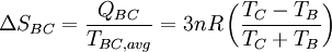
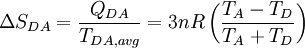
then it can be proven that for any cyclic process,

$\oint dS = \oint {dQ \over T} = 0.$

Demonstration

Part 1

Draw a rectangle on a P-V diagram, such that the top and bottom are horizontal isobaric processes and the left and right are vertical isochoric processes. Such a rectangle should be made really small, so that change in temperature can be averaged out, and so that the cycle will enclose an area $Δarea$ .

Let the top left corner be labeled A, then label the rest of the corners clockwise starting from A as ABCD.

Assume that the system is a monatomic gas. Then

W A B = P A (V B - V A)

$Q_{AB} = {5 \over 2} n R (T_B - T_A)$

$\Delta S_{AB} = {Q_{AB} \over T_{AB, avg}} = 5 n R \left( { T_B - T_A \over T_B + T_A } \right)$

Process BC:

W B C = 0

$Q_{BC} = {3 \over 2} n R (T_C - T_B)$

$\Delta S_{BC} = {Q_{BC} \over T_{BC, avg}} = 3 n R \left( { T_C - T_B \over T_C + T_B } \right)$

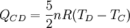
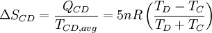
Process CD:

W C D = P C (V A - V C)

$Q_{CD} = {5 \over 2} n R (T_D - T_C)$

$\Delta S_{CD} = {Q_{CD} \over T_{CD, avg}} = 5 n R \left( {T_D - T_C \over T_D + T_C } \right)$

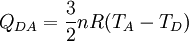
Process DA:

W D A = 0

$Q_{DA} = {3 \over 2} n R (T_A - T_D)$

$\Delta S_{DA} = {Q_{DA} \over T_{DA, avg}} = 3 n R \left( {T_A - T_D \over T_A + T_D } \right)$

Process ABCDA (cyclic):

$\Delta S_{cyc} = 5 n R \left( {T_B - T_A \over T_B + T_A } \right) + 3 n R \left( {T_C - T_B \over T_C + T_B } \right) + 5 n R \left( {T_D - T_C \over T_D + T_C } \right) + 3 n R \left( { T_A - T_D \over T_A + T_D } \right)$

$\Delta S_{cyc} = 5 n R \left( {V_C - V_A \over V_C + V_A } \right) + 3 n R \left( {P_C - P_A \over P_C + P_A } \right) + 5 n R \left( {V_A - V_C \over V_A + V_C } \right) + 3 n R \left( { P_A - P_C \over P_A + P_C } \right)$

$\Delta S_{cyc} = 5 n R \left( {V_C - V_A \over V_C + V_A } \right) + 3 n R \left( {P_C - P_A \over P_C + P_A } \right) - 5 n R \left( {V_C - V_A \over V_C + V_A } \right) - 3 n R \left( { P_C - P_A \over P_C + P_A } \right)$

$\Delta S_{cyc} = 0 \qquad$

Part 2

Any loop can be broken up into a rectangular grid of differential areas. The line integral of the entire loop is equal to the sum of the line integrals of each of the constituent differential areas. Let all these integrals be done clockwise. Then any pair of adjacent differential areas will be sharing a process as a common border, but one area will add that process in one direction while the adjacent area adds that process in the reverse direction, so that process is cancelled out. Therefore all processes internal to the loop cancel each other out (see Green's theorem), and the result of the summation is equal to the line integral of the contour of the loop:

ΔS(contour) =	∑	ΔS(Δarea) =	∑	0 = 0
	area		area

Q.E.D.

Conclusion

The fact that entropy is a state function is what puts entropy on the map (the P-V diagram).

References

Halliday, Resnick & Walker. Fundamentals of Physics, 5th edition. John Wiley & Sons, 1997. Chapter 21, Entropy and the Second Law of Thermodynamics.