To use all functions of this page, please activate cookies in your browser.
My watch list
my.chemeurope.com
my.chemeurope.com
With an accout for my.chemeurope.com you can always see everything at a glance – and you can configure your own website and individual newsletter.
- My watch list
- My saved searches
- My saved topics
- My newsletter
Implicit solvationImplicit solvation (sometimes known as continuum solvation) is a method of representing solvent as a continuous medium instead of individual “explicit” solvent molecules most often used in molecular dynamics simulations and in other applications of molecular mechanics. The method is often applied to estimate free energy of solute-solvent interactions in structural and chemical processes, such as folding or conformational transitions of proteins, DNA, RNA, and polysaccharides, association of biological macromolecules with ligands, or transport of drugs across biological membranes. The implicit solvation model is justified in liquids, where the potential of mean force can be applied to approximate the averaged behavior of many highly dynamic solvent molecules. However, the interiors of biological membranes or proteins can also be considered as media with specific solvation or dielectric properties. These media are continuous but not necessarily uniform, since their properties can be described by different analytical functions, such as “polarity profiles” of lipid bilayers.[1] There are two basic types of implicit solvent methods: models based on accessible surface areas (ASA) that were historically the first, and more recent continuum electrostatics models, although various modifications and combinations of the different methods are possible. The accessible surface area (ASA) method is based on experimental linear relations between Gibbs free energy of transfer and the surface area of a solute molecule.[2] This method operates directly with free energy of solvation, unlike molecular mechanics or electrostatic methods that include only the enthalpic component of free energy. The continuum representation of solvent also significantly improves the computational speed and reduces errors in statistical averaging that arise from incomplete sampling of solvent conformations,[3] so that the energy landscapes obtained with implicit and explicit solvent are different.[4] Although the implicit solvent model is useful for simulations of biomolecules, this is an approximate method with certain limitations and problems related to parameterization and treatment of ionization effects. Product highlight
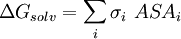
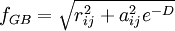
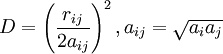
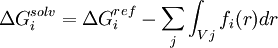
Accessible surface area based methodThe free energy of solvation of a solute molecule in the simplest ASA-based method is given by: where ASAi is accessible surface area of atom i, and σi is solvation parameter of atom i, i.e. a contribution to the free energy of solvation of the particular atom i per surface unit area. The required solvation parameters for different types of atoms (C, N, O, S, etc.) are usually determined by least squares fit of the calculated and experimental transfer free energies for a series of organic compounds. The experimental energies are determined from partition coefficients of these compounds between different solutions or media using standard mole concentrations of the solutes [5] [6]. It is noteworthy that solvation energy is free energy required to transfer a solute molecule from a solvent to “vacuum” (gas phase). This solvation energy can supplement the intramolecular energy in vacuum calculated in molecular mechanics. Therefore, the required atomic solvation parameters were initially derived from water-gas partition data [7]. However, the dielectric properties of proteins and lipid bilayers are much more similar to those of nonpolar solvents than to vacuum. Newer parameters have therefore been derived from water-octanol partition coefficients [8] or other similar data. Such parameters actually describe transfer energy between two condensed media or the difference of two solvation energies. Poisson-BoltzmannAlthough this equation has solid theoretical justification, it is computationally expensive to calculate without approximations. The Poisson-Boltzmann equation (PB) describes the electrostatic environment of a solute in a solvent containing ions. It can be written in cgs units as: where A number of numerical Poisson-Boltzmann equation solvers of varying generality and efficiency have been developed,[10][11][12] including one application with a specialized computer hardware platform.[13] However, performance from PB solvers does not yet equal that from the more commonly used generalized Born approximation.[14] Generalized BornThe Generalized Born (GB) model is an approximation to the exact (linearized) Poisson-Boltzmann equation. It is based on modeling the protein as a sphere whose internal dielectric constant differs from the external solvent. The model has the following functional form: where and
where ε0 is the permittivity of free space, ε is the dielectric constant of the solvent being modeled, qi is the electrostatic charge on particle i, rij is the distance between particles i and j, and ai is a quantity (with the dimension of length) known as the effective Born radius.[15] The effective Born radius of an atom characterizes its degree of burial inside the solute; qualitatively it can be thought of as the distance from the atom to the molecular surface. Accurate estimation of the effective Born radii is critical for the GB model .[16] GBSAGBSA is simply a Generalized Born model augmented with the hydrophobic solvent accessible surface area SA term. It is among the most commonly used implicit solvent model combinations. The use of this model in the context of molecular mechanics is known as MM/GBSA. Although this formulation has been shown to successfully identify the native states of short peptides with well-defined tertiary structure[17], the conformational ensembles produced by GBSA models in other studies differ significantly from those produced by explicit solvent and do not identify the protein's native state.[4] In particular, salt bridges are overstabilized, possibly due to insufficient electrostatic screening, and a higher-than-native alpha helix population was observed. Variants of the GB model have also been developed to approximate the electrostatic environment of membranes, which have had some success in folding the transmembrane helices of integral membrane proteins.[18] Ad-hoc fast solvation modelsAnother possibility is to use ad-hoc quick strategies to estimate solvation free energy. A first generation of fast implicit solvents is based on the calculation of a per-atom solvent accessible surface area. For each of group of atom types, a different parameter scales its contribution to solvation ("ASA-based model" described above). [19] Another strategy is implemented for the CHARMM19 force-field and is called EEF1 [20]. EEF1 is based on a Gaussian-shaped solvent exclusion. The solvation free energy is The reference solvation free energy of i corresponds to a suitably chosen small molecule in which group i is essentially fully solvent-exposed. The integral is over the volume Vj of group j and the summation is over all groups j around i. EEF1 additionally utilizes a distance-dependent (non-constant) dielectric, and ionic side-chains of proteins are simply neutralized. It is only 50% slower than a vacuum simulation. This model was later augmented with the hydrophobic effect and called Charmm19/SASA. [21] Hybrid implicit/explicit solvation modelsIt is possible to include a layer or sphere of water molecules around the solute, and model the bulk with an implicit solvent. Such an approach is proposed by M.S. Lee and coworkers. [22] The bulk solvent is modeled with a Generalized Born approach and the multi-grid method used for Coulombic pairwise particle interactions. It is reported to be faster than a full explicit solvent simulation with the particle mesh Ewald (PME) method of electrostatic calculation. Effects not accounted forThe hydrophobic effectModels like PB and GB allow estimation of the mean electrostatic free energy but do not account for entropic effects arising from solute-imposed constraints on the organization of the water or solvent molecules. This is known as the hydrophobic effect and is a major factor in the folding process of globular proteins with hydrophobic cores. Implicit solvation models may be augmented with a term that accounts for the hydrophobic effect. The most popular way to do this is by taking the solvent accessible surface area (SASA) as a proxy of the extent of the hydrophobic effect. Most authors place the extent of this effect between 5 and 45 cal/(Å2 mol). [23] Note that this surface area pertains to the solute, while the hydrophobic effect is entropic in nature and occurs on the side of the solvent. ViscosityImplicit solvent models such as PB, GB, and SASA lack the viscosity that water molecules impart by randomly colliding and impeding the motion of solutes through their van der Waals repulsion. In many cases, this is desirable because it makes sampling of configurations and phase space much faster. This acceleration means that more configurations are visited per simulated nanosecond, on top of whatever CPU acceleration is achieved in comparison to explicit solvent. But it can lead to misleading results when kinetics are of interest. Viscosity may be added back by using Langevin dynamics instead of Hamiltonian dynamics and choosing an appropriate damping constant for the particular solvent. [24] Hydrogen-bonds with waterThe average energetic contribution of protein-water hydrogen bonds may be reproduced with an implicit solvent. However, the directionality of these hydrogen bonds will be missing. Problems and limitationsAll implicit solvation models rest on the simple idea that nonpolar atoms of a solute tend to cluster together or occupy nonpolar media, whereas polar and charged groups of the solute tend to remain in water. However, it is important to properly balance the opposite energy contributions from different types of atoms. Several important points have been discussed and investigated over the years. Choice of model solventIt has been noted that wet octanol solution is a poor approximation of proteins or biological membranes because it contains ~2M of water, and that cyclohexane would be a much better approximation [25]. Investigation of passive permeability barriers for different compounds across lipid bilayers led to conclusion that 1,9-decadiene can serve as a good approximations of the bilayer interior [26], whereas octanol was a very poor approximation [27]. A set of solvation parameters derived for protein interior from protein engineering data was also different from octanol scale: it was close to cyclohexane scale for nonpolar atoms but intermediate between cyclohexane and octanol scales for polar atoms [28]. Thus, different atomic solvation parameters should be applied for modeling of protein folding and protein-membrane binding. This issue remains controversial. The original idea of the method was to derive all solvation parameters directly from experimental partition coefficients of organic molecules, which allows calculation of solvation free energy. However, some of the recently developed electrostatic models use ad hoc values of 20 or 40 cal/(Å2 mol) for all types of atoms. The non-existent “hydrophobic” interactions of polar atoms are overridden by large electrostatic energy penalties in such models. Solid-state applicationsStrictly speaking, ASA-based models should only be applied to describe solvation, i.e. energetics of transfer between liquid or uniform media. It is possible to express van der Waals interaction energies in the solid state in the surface energy units. This was sometimes done for interpreting protein engineering and ligand binding energetics [29], which leads to “solvation” parameter for aliphatic carbon of ~40 cal/(Å2 mol) [30], which is 2 times bigger than ~20 cal/(Å2 mol) obtained for transfer from water to liquid hydrocarbons, because the parameters derived by such fitting represent sum of the hydrophobic energy (i.e. 20 cal/Å2 mol) and energy of van der Waals attractions of aliphatic groups in the solid state, which corresponds to fusion enthalpy of alkanes [28]. Unfortunately, the simplified ASA-based model can not capture the "specific" distance-dependent interactions between different types of atoms in the solid state which are responsible for clustering of atoms with similar polarities in protein structures and molecular crystals. Parameters of such interatomic interactions, together with atomic solvation parameters for the protein interior, have been approximately derived from protein engineering data [28]. The implicit solvation model breaks down when solvent molecules associate strongly with binding cavities in a protein, so that the protein and the solvent molecules form a continuous solid body. [31]. On the other hand, this model can be successfully applied for describing transfer from water to the fluid lipid bilayer [32]. Importance of extensive testingMore testing is needed to evaluate the performance of different implicit solvation models and parameter sets. They are often tested only for a small set of molecules with very simple structure, such as hydrophobic and amphiphilic α-helices. This method was rarely tested for hundreds of protein structures[32]. Treatment of ionization effectsIonization of charged groups has been neglected in continuum electrostatic models of implicit solvation, as well as in standard molecular mechanics and molecular dynamics. The transfer of an ion from water to a nonpolar media with dielectric constant of ~3 (lipid bilayer) or 4 to 10 (interior of proteins) costs significant energy, as follows from Born equation and experiments. However, since the charged protein residues are ionizable, they simply lose their charges in the nonpolar environment, which costs relatively little at the neutral pH: ~4 to 7 kcal/mol for Asp, Glu, Lys, and Arg amino acid residues, according to the Henderson-Hasselbalch equation, ΔG=2.3RT(pH-pK). The low energetic costs of such ionization effects have indeed been observed for protein mutants with buried ionizable residues [33] and hydrophobic α-helical peptides in membranes with a single ionizable residue in the middle [34]. However, all electrostatic methods, such as PB, GB, or GBSA assume that ionizable groups remain charged in the nonpolar environments, which leads to grossly overestimated electrostatic energy. In the simplest accessible surface area-based models, this problem was treated using different solvation parameters for charged atoms or Henderson-Hasselbalch equation with some modifications [32]. However even the latter approach does not solve the problem. Charged residues can remain charged even in the nonpolar environment if they are invloved in intramolecular ion pairs and H-bonds. Thus, the energetic penalties can be overestimated even using the Henderson-Hasselbalch equation. More rigorous theoretical methods describing such ionization effects have been developed [35], and there are ongoing efforts to incorporate such methods into the implicit solvation models [36] References
See also
Categories: Molecular modelling | Computational chemistry | Molecular dynamics | Protein structure |
|
| This article is licensed under the GNU Free Documentation License. It uses material from the Wikipedia article "Implicit_solvation". A list of authors is available in Wikipedia. |


![\vec{\nabla}\left[\epsilon(\vec{r})\vec{\nabla}\Psi(\vec{r})\right] = -4\pi\rho^{f}(\vec{r}) - 4\pi\sum_{i}c_{i}^{\infty}z_{i}q\lambda(\vec{r})e^{\frac{-z_{i}q\Psi(\vec{r})}{kT}}](images/math/e/a/2/ea2ab8bd373070a7fb81dc986a9ca431.png)
 represents the position-dependent dielectric,
  represents the electrostatic potential,
  represents the charge density of the solute,
  represents the concentration of the ion i at a distance of infinity from the solute,
  is a factor for the position-dependent accessibility of position r to the ions in solution (often set to uniformly 1). If the potential is not large, the equation can be linearized to be solved more efficiently.
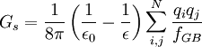
Last viewed


