To use all functions of this page, please activate cookies in your browser.
My watch list
my.chemeurope.com
my.chemeurope.com
With an accout for my.chemeurope.com you can always see everything at a glance – and you can configure your own website and individual newsletter.
- My watch list
- My saved searches
- My saved topics
- My newsletter
Statistical mechanics
Statistical mechanics is the application of probability theory, which includes mathematical tools for dealing with large populations, to the field of mechanics, which is concerned with the motion of particles or objects when subjected to a force. Statistical mechanics, sometimes called statistical physics, can be viewed as a subfield of physics and chemistry. It provides a framework for relating the microscopic properties of individual atoms and molecules to the macroscopic or bulk properties of materials that can be observed in everyday life, therefore explaining thermodynamics as a natural result of statistics and mechanics (classical and quantum) at the microscopic level. In particular, it can be used to calculate the thermodynamic properties of bulk materials from the spectroscopic data of individual molecules. This ability to make macroscopic predictions based on microscopic properties is the main asset of statistical mechanics over thermodynamics. Both theories are governed by the second law of thermodynamics through the medium of entropy. However, entropy in thermodynamics can only be known empirically, whereas in statistical mechanics, it is a function of the distribution of the system on its micro-states. Product highlight
Fundamental postulateThe fundamental postulate in statistical mechanics (also known as the equal a priori probability postulate) is the following:
This postulate is a fundamental assumption in statistical mechanics - it states that a system in equilibrium does not have any preference for any of its available microstates. Given Ω microstates at a particular energy, the probability of finding the system in a particular microstate is p = 1/Ω. This postulate is necessary because it allows one to conclude that for a system at equilibrium, the thermodynamic state (macrostate) which could result from the largest number of microstates is also the most probable macrostate of the system. The postulate is justified in part, for classical systems, by Liouville's theorem (Hamiltonian), which shows that if the distribution of system points through accessible phase space is uniform at some time, it remains so at later times. Similar justification for a discrete system is provided by the mechanism of detailed balance. This allows for the definition of the information function (in the context of information theory): When all rhos are equal, I is minimal, which reflects the fact that we have minimal information about the system. When our information is maximal, i.e. one rho is equal to one and the rest to zero (we know what state the system is in), the function is maximal. This "information function" is the same as the reduced entropic function in thermodynamics. Microcanonical ensembleSince the second law of thermodynamics applies to isolated systems, the first case investigated will correspond to this case. The Microcanonical ensemble describes an isolated system. The entropy of such a system can only increase, so that the maximum of its entropy corresponds to an equilibrium state for the system. Because an isolated system keeps a constant energy, the total energy of the system does not fluctuate. Thus, the system can access only those of its micro-states that correspond to a given value E of the energy. The internal energy of the system is then strictly equal to its energy. Let us call
Canonical ensembleInvoking the concept of the canonical ensemble, it is possible to derive the probability
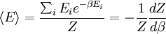
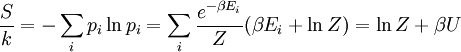
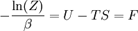
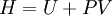
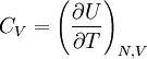
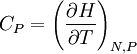
The temperature where To sum up, the probability of finding a system at temperature Thermodynamic ConnectionThe partition function can be used to find the expected (average) value of any microscopic property of the system, which can then be related to macroscopic variables. For instance, the expected value of the microscopic energy implies, together with the interpretation of The entropy can be calculated by (see Shannon entropy) which implies that is the Free energy of the system or in other words, Having microscopic expressions for the basic thermodynamic potentials The treatment in this section assumes no exchange of matter (i.e. fixed mass and fixed particle numbers). However, the volume of the system is variable which means the density is also variable. This probability can be used to find the average value, which corresponds to the macroscopic value, of any property, J, that depends on the energetic state of the system by using the formula: where Subsequently, these equations can be combined with known thermodynamic relationships between
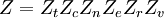
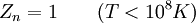
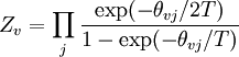
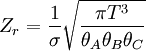
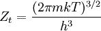
To clarify, this is not a grand canonical ensemble. It is often useful to consider the energy of a given molecule to be distributed among a number of modes. For example, translational energy refers to that portion of energy associated with the motion of the center of mass of the molecule. Configurational energy refers to that portion of energy associated with the various attractive and repulsive forces between molecules in a system. The other modes are all considered to be internal to each molecule. They include rotational, vibrational, electronic and nuclear modes. If we assume that each mode is independent (a questionable assumption) the total energy can be expressed as the sum of each of the components: Where the subscripts If we can assume all these modes are completely uncoupled and uncorrelated, so all these factors are in a probability sense completely independent, then Thus a partition function can be defined for each mode. Simple expressions have been derived relating each of the various modes to various measurable molecular properties, such as the characteristic rotational or vibrational frequencies. Expressions for the various molecular partition functions are shown in the following table.
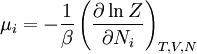
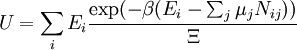
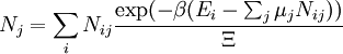
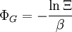
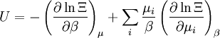
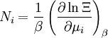
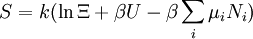
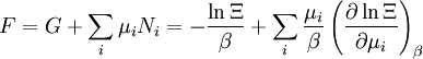
These equations can be combined with those in the first table to determine the contribution of a particular energy mode to a thermodynamic property. For example the "rotational pressure" could be determined in this manner. The total pressure could be found by summing the pressure contributions from all of the individual modes, ie: Grand canonical ensembleIf the system under study is an open system, (matter can be exchanged), but particle number is not conserved, we would have to introduce chemical potentials, μj, j=1,...,n and replace the canonical partition function with the grand canonical partition function: where Nij is the number of jth species particles in the ith configuration. Sometimes, we also have other variables to add to the partition function, one corresponding to each conserved quantity. Most of them, however, can be safely interpreted as chemical potentials. In most condensed matter systems, things are nonrelativistic and mass is conserved. However, most condensed matter systems of interest also conserve particle number approximately (metastably) and the mass (nonrelativistically) is none other than the sum of the number of each type of particle times its mass. Mass is inversely related to density, which is the conjugate variable to pressure. For the rest of this article, we will ignore this complication and pretend chemical potentials don't matter. See grand canonical ensemble. Let's rework everything using a grand canonical ensemble this time. The volume is left fixed and does not figure in at all in this treatment. As before, j is the index for those particles of species j and i is the index for microstate i:
Equivalence between descriptions at the thermodynamic limitAll the above descriptions differ in the way they allow the given system to fluctuate between its configurations. In the micro-canonical ensemble, the system exchanges no energy with the outside world, and is therefore not subject to energy fluctuations, while in the canonical ensemble, the system is free to exchange energy with the outside in the form of heat. In the thermodynamic limit, which is the limit of large systems, fluctuations become negligible, so that all these descriptions converge to the same description. In other words, the macroscopic behavior of a system does not depend on the particular ensemble used for its description. Given these considerations, the best ensemble to choose for the calculation of the properties of a macroscopic system is that ensemble which allows the result be most easily derived. Random walkersThe study of long chain polymers has been a source of problems within the realms of statistical mechanics since about the 1950's. One of the reasons however that scientists were interested in their study is that the equations governing the behaviour of a polymer chain were independent of the chain chemistry. What is more, the governing equation turns out to be a random (diffusive) walk in space. Indeed, Schrodinger's equation is itself a diffusion equation in imaginary time, t' = it. Random walks in timeThe first example of a random walk is one in space, whereby a particle undergoes a random motion due to external forces in its surrounding medium. A typical example would be a pollen grain in a beaker of water. If one could somehow "dye" the path the pollen grain has taken, the path observed is defined as a random walk. Consider a toy problem, of a train moving along a 1D track in the x-direction. Suppose that the train moves either a distance of + or - a fixed distance b, depending on whether a coin lands heads or tails when flipped. Lets start by considering the statistics of the steps the toy train takes (where Si is the ith step taken):
The second quantity is known as the correlation function. The delta is the kronecker delta which tells us that if the indices i and j are different, then the result is 0, but if i = j then the kronecker delta is 1, so the correlation function returns a value of b2. This makes sense, because if i = j then we are considering the same step. Rather trivially then it can be shown that the average displacement of the train on the x-axis is 0;
As stated
From the diffusion equation it can be shown that the distance a diffusing particle moves in a media is proportional to the root of the time the system has been diffusing for, where the proportionality constant is the root of the diffusion constant. The above relation, although cosmetically different reveals similar physics, where N is simply the number of steps moved (is loosely connected with time) and b is the characteristic step length. As a consequence we can consider diffusion as a random walk process. Random walks in spaceRandom walks in space can be thought of as snapshots of the path taken by a random walker in time. One such example is the spatial configuration of long chain polymers. There are two types of random walk in space: self-avoiding random walks, where the links of the polymer chain interact and do not overlap in space, and pure random walks, where the links of the polymer chain are non-interacting and links are free to lie on top of one another. The former type is most applicable to physical systems, but their solutions are harder to get at from first principles. By considering a freely jointed, non-interacting polymer chain, the end-to-end vector is Assuming, as stated, that that distribution of end-to-end vectors for a very large number of identical polymer chains is gaussian, the probability distribution has the following form
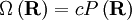
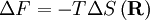
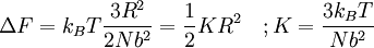
What use is this to us? Recall that according to the principle of equally likely a priori probabilities, the number of microstates, Ω, at some physical value is directly proportional to the probability distribution at that physical value, viz;
where c is an arbitrary proportionality constant. Given our distribution function, there is a maxima corresponding to See also
References
Categories: Statistical mechanics | Thermodynamics |
|||||||||||||||||||||||||||||||||||||||||||||||||||||||||||||||||||||||||||||||||||||
| This article is licensed under the GNU Free Documentation License. It uses material from the Wikipedia article "Statistical_mechanics". A list of authors is available in Wikipedia. | |||||||||||||||||||||||||||||||||||||||||||||||||||||||||||||||||||||||||||||||||||||


 the number of micro-states corresponding to this value of the system's energy. The macroscopic state of maximal entropy for the system is the one in which all micro-states are equally likely to occur during the system's fluctuations.
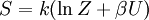
 is the system entropy,
 is
is  that a macroscopic system in
  :
:
 ,
,
 arises from the fact that the system is in thermal equilibrium with its environment. The probabilities of the various microstates must add to one, and the normalization factor in the denominator is the canonical
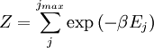
 th microstate of the system. The partition function is a measure of the number of states accessible to the system at a given temperature. The article
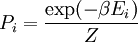
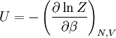
 is interpreted as the microscopic definition of the thermodynamic variable internal energy
  ., and can be obtained by taking the derivative of the partition function with respect to the temperature. Indeed,
 as
as 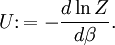

 (
(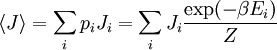
 is the average value of property
  . This equation can be applied to the internal energy,
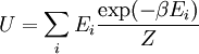
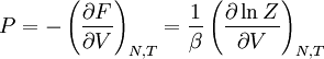
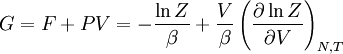
 to arrive at an expression for pressure in terms of only temperature, volume and the partition function. Similar relationships in terms of the partition function can be derived for other thermodynamic properties as shown in the following table; see also the detailed explanation in
configuration integral.
to arrive at an expression for pressure in terms of only temperature, volume and the partition function. Similar relationships in terms of the partition function can be derived for other thermodynamic properties as shown in the following table; see also the detailed explanation in
configuration integral.


 ,
,  ,
,  ,
,  ,
,  , and
, and  correspond to translational, configurational, nuclear, electronic, rotational and vibrational modes, respectively. The relationship in this equation can be substituted into the very first equation to give:


![\Xi(V,T,\mu) = \sum_i \exp\left(\beta \left[\sum_{j=1}^n \mu_j N_{ij}-E_i\right ]\right)](images/math/f/a/4/fa4a0a546cb56b26e20a56be1480d439.png)
 ; due to a priori equal probabilities

 is 0, so the sum of 0 is still 0.
It can also be shown, using the same method demonstrated above, to calculate the root mean square value of problem. The result of this calculation is given below
is 0, so the sum of 0 is still 0.
It can also be shown, using the same method demonstrated above, to calculate the root mean square value of problem. The result of this calculation is given below

 where
where  is the vector position of the i-th link in the chain.
As a result of the central limit theorem, if N >> 1 then the we expect a Gaussian distribution for the end-to-end vector. We can also make statements of the statistics of the links themselves;
is the vector position of the i-th link in the chain.
As a result of the central limit theorem, if N >> 1 then the we expect a Gaussian distribution for the end-to-end vector. We can also make statements of the statistics of the links themselves;
 ; by the isotropy of space
  ; all the links in the chain are uncorrelated with one another
 and
and 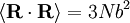 . Notice this last result is the same as that found for random walks in time.
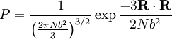
 . Physically this amounts to there being more microstates which have an end-to-end vector of 0 than any other microstate. Now by considering
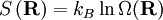

Last viewed


